Assignment 3: Mapping Census Data

library(tidycensus)

Warning: package 'tidycensus' was built under R version 4.5.3

library(tigris)

Warning: package 'tigris' was built under R version 4.5.3

To enable caching of data, set `options(tigris_use_cache = TRUE)`
in your R script or .Rprofile.

library(sf)

Warning: package 'sf' was built under R version 4.5.3

Linking to GEOS 3.14.1, GDAL 3.12.1, PROJ 9.7.1; sf_use_s2() is TRUE

library(dplyr)

Warning: package 'dplyr' was built under R version 4.5.3


Attaching package: 'dplyr'

The following objects are masked from 'package:stats':

    filter, lag

The following objects are masked from 'package:base':

    intersect, setdiff, setequal, union

library(ggplot2)

Warning: package 'ggplot2' was built under R version 4.5.3

library(readr)

Warning: package 'readr' was built under R version 4.5.3

options(tigris_use_cache = TRUE)

# 1) API key (c5c7d8f0315d0bb7a67c1a7549772a162a4eecfa)
# census_api_key("c5c7d8f0315d0bb7a67c1a7549772a162a4eecfa", install = FALSE)

# 2) Explore variables
vars <- load_variables(2023, "acs5", cache = TRUE)
# View a few example codes
vars |> dplyr::filter(grepl("^B19", name)) |> dplyr::slice_head(n = 10)

# A tibble: 10 × 4
   name        label                                concept            geography
   <chr>       <chr>                                <chr>              <chr>    
 1 B19001A_001 Estimate!!Total:                     Household Income … tract    
 2 B19001A_002 Estimate!!Total:!!Less than $10,000  Household Income … tract    
 3 B19001A_003 Estimate!!Total:!!$10,000 to $14,999 Household Income … tract    
 4 B19001A_004 Estimate!!Total:!!$15,000 to $19,999 Household Income … tract    
 5 B19001A_005 Estimate!!Total:!!$20,000 to $24,999 Household Income … tract    
 6 B19001A_006 Estimate!!Total:!!$25,000 to $29,999 Household Income … tract    
 7 B19001A_007 Estimate!!Total:!!$30,000 to $34,999 Household Income … tract    
 8 B19001A_008 Estimate!!Total:!!$35,000 to $39,999 Household Income … tract    
 9 B19001A_009 Estimate!!Total:!!$40,000 to $44,999 Household Income … tract    
10 B19001A_010 Estimate!!Total:!!$45,000 to $49,999 Household Income … tract

# 3) Parameters (EDIT ME)
state_abbr <- "CA"
geo_level  <- "county"   # options: state, county, tract, block group
my_vars    <- c(income = "B19013_001", poverty = "B17001_002")
year_acs   <- 2023
survey     <- "acs5"

# 4) Download
acs <- get_acs(
  geography = geo_level,
  variables = my_vars,
  state = state_abbr,
  year = year_acs,
  survey = survey,
  geometry = TRUE
)

Getting data from the 2019-2023 5-year ACS

library(tidycensus)
# 5) Wide format for convenience
acs_wide <- acs |>
  tidyr::pivot_wider(
    id_cols = c(GEOID, NAME, geometry),
    names_from = variable,
    values_from = c(estimate, moe)
  )

# 6) Map (edit titles/theme)
ggplot(acs_wide) +
  geom_sf(aes(fill = estimate_income), color = NA) +
  scale_fill_viridis_c(name = "Median HH Income") +
  labs(title = paste0("ACS ", year_acs, " 5-year: Median Income — ", state_abbr, " (", geo_level, ")"),
       caption = "Source: U.S. Census Bureau via tidycensus") +
  theme_minimal()

# 7) Table (top/bottom by poverty count)
top10 <- acs_wide |>
  arrange(desc(estimate_poverty)) |>
  select(NAME, estimate_poverty, moe_poverty) |>
  slice_head(n = 10)

bottom10 <- acs_wide |>
  arrange(estimate_poverty) |>
  select(NAME, estimate_poverty, moe_poverty) |>
  slice_head(n = 10)

top10

Simple feature collection with 10 features and 3 fields
Geometry type: MULTIPOLYGON
Dimension:     XY
Bounding box:  xmin: -122.3423 ymin: 32.53444 xmax: -114.1312 ymax: 38.7364
Geodetic CRS:  NAD83
# A tibble: 10 × 4
   NAME                   estimate_poverty moe_poverty                  geometry
   <chr>                             <dbl>       <dbl>        <MULTIPOLYGON [°]>
 1 Los Angeles County, C…          1322476       15552 (((-118.6044 33.47855, -…
 2 San Diego County, Cal…           330602        7963 (((-117.596 33.38779, -1…
 3 Orange County, Califo…           296493        8509 (((-118.1146 33.74461, -…
 4 San Bernardino County…           291226        9076 (((-117.8025 33.97555, -…
 5 Riverside County, Cal…           266955        8729 (((-117.6763 33.88882, -…
 6 Sacramento County, Ca…           197472        6775 (((-121.8625 38.06795, -…
 7 Fresno County, Califo…           185717        5965 (((-120.9094 36.7477, -1…
 8 Kern County, Californ…           168825        6993 (((-120.1944 35.78936, -…
 9 Alameda County, Calif…           149752        4801 (((-122.3423 37.80556, -…
10 Santa Clara County, C…           128470        5622 (((-122.2027 37.36305, -…

bottom10

Simple feature collection with 10 features and 3 fields
Geometry type: MULTIPOLYGON
Dimension:     XY
Bounding box:  xmin: -124.256 ymin: 35.78669 xmax: -115.648 ymax: 42.00076
Geodetic CRS:  NAD83
# A tibble: 10 × 4
   NAME                   estimate_poverty moe_poverty                  geometry
   <chr>                             <dbl>       <dbl>        <MULTIPOLYGON [°]>
 1 Alpine County, Califo…              209          98 (((-120.0724 38.70277, -…
 2 Sierra County, Califo…              325         202 (((-121.0575 39.53999, -…
 3 Mono County, Californ…             1441         480 (((-119.6489 38.28912, -…
 4 Modoc County, Califor…             1717         357 (((-121.4572 41.94994, -…
 5 Inyo County, Californ…             1928         439 (((-118.79 37.39403, -11…
 6 Plumas County, Califo…             2075         538 (((-121.497 40.43702, -1…
 7 Colusa County, Califo…             2332         598 (((-122.7851 39.38298, -…
 8 Mariposa County, Cali…             2347         449 (((-120.3944 37.67504, -…
 9 Trinity County, Calif…             2830         755 (((-123.6224 40.9317, -1…
10 Del Norte County, Cal…             2900         589 (((-124.2175 41.95081, -…

# 8) Save outputs (optional)
# readr::write_csv(st_drop_geometry(acs_wide), "acs_data.csv")

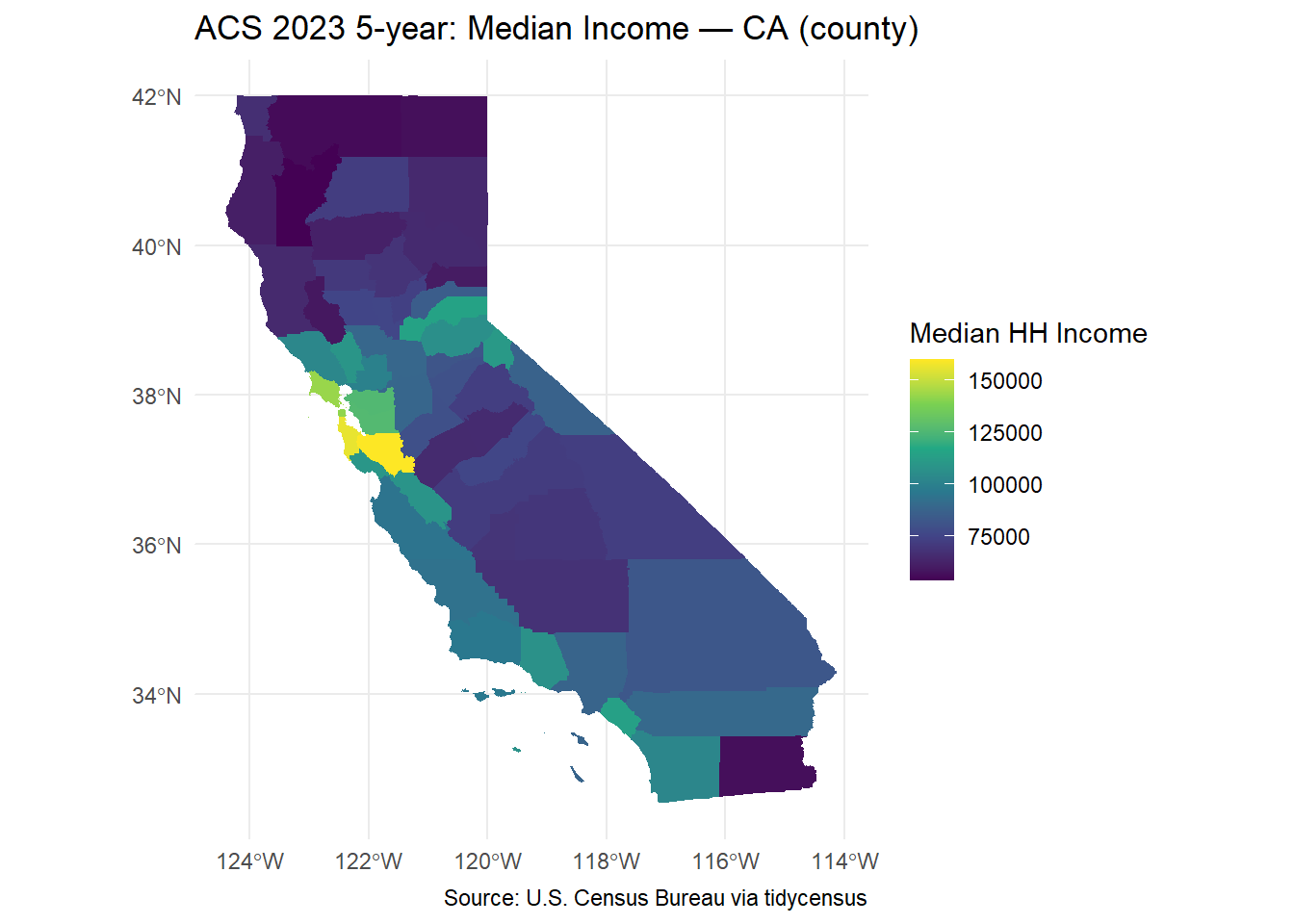
In this assignment, I present data on median household incomes in the state of California by county. The yellow-highlighted counties represent the areas with the highest incomes, whereas the dark-blue areas represent the counties with the lowest incomes.

The next visualization shows the top 10 highest-income counties in California, such as Los Angeles, San Diego, and Orange County. Then, I present the top 10 counties with the lowest incomes, which include Mariposa, Trinity, and Del Norte County.