Assignment 3: ML Exercise

Lab_ML01.R

library(haven)        # Read Stata files

Warning: package 'haven' was built under R version 4.5.2

library(tidyverse)    # Data wrangling and visualization

Warning: package 'tidyverse' was built under R version 4.5.3

Warning: package 'ggplot2' was built under R version 4.5.3

Warning: package 'tidyr' was built under R version 4.5.3

Warning: package 'readr' was built under R version 4.5.3

Warning: package 'dplyr' was built under R version 4.5.3

Warning: package 'lubridate' was built under R version 4.5.2

── Attaching core tidyverse packages ──────────────────────── tidyverse 2.0.0 ──
✔ dplyr     1.2.1     ✔ readr     2.2.0
✔ forcats   1.0.0     ✔ stringr   1.5.1
✔ ggplot2   4.0.2     ✔ tibble    3.3.0
✔ lubridate 1.9.4     ✔ tidyr     1.3.2
✔ purrr     1.1.0     
── Conflicts ────────────────────────────────────────── tidyverse_conflicts() ──
✖ dplyr::filter() masks stats::filter()
✖ dplyr::lag()    masks stats::lag()
ℹ Use the conflicted package (<http://conflicted.r-lib.org/>) to force all conflicts to become errors

library(GGally)       # Pairs plots

Warning: package 'GGally' was built under R version 4.5.2

library(cluster)      # Clustering

Warning: package 'cluster' was built under R version 4.5.2

library(factoextra)   # Visualize clusters and PCA

Warning: package 'factoextra' was built under R version 4.5.2

Welcome to factoextra!
Want to learn more? See two factoextra-related books at https://www.datanovia.com/en/product/practical-guide-to-principal-component-methods-in-r/

library(rpart)        # Decision trees

Warning: package 'rpart' was built under R version 4.5.2

library(rpart.plot)   # Plot decision trees

Warning: package 'rpart.plot' was built under R version 4.5.2

library(randomForest) # Random forest

Warning: package 'randomForest' was built under R version 4.5.3

randomForest 4.7-1.2
Type rfNews() to see new features/changes/bug fixes.

Attaching package: 'randomForest'

The following object is masked from 'package:dplyr':

    combine

The following object is masked from 'package:ggplot2':

    margin

library(caret)        # Model training and evaluation

Warning: package 'caret' was built under R version 4.5.3

Loading required package: lattice

Attaching package: 'caret'

The following object is masked from 'package:purrr':

    lift

library(e1071)        # SVM and Naive Bayes

Warning: package 'e1071' was built under R version 4.5.2

Attaching package: 'e1071'

The following object is masked from 'package:ggplot2':

    element

# Load data
TEDS_2016 <- read_stata("https://github.com/datageneration/home/blob/master/DataProgramming/data/TEDS_2016.dta?raw=true")


# ============================================================================
# PART I: EXPLORATORY DATA ANALYSIS
# ============================================================================

# ----------------------------------------------------------------------------
# Q1. Data overview
# ----------------------------------------------------------------------------

dim(TEDS_2016)

[1] 1690   54

names(TEDS_2016)

 [1] "District"        "Sex"             "Age"             "Edu"            
 [5] "Arear"           "Career"          "Career8"         "Ethnic"         
 [9] "Party"           "PartyID"         "Tondu"           "Tondu3"         
[13] "nI2"             "votetsai"        "green"           "votetsai_nm"    
[17] "votetsai_all"    "Independence"    "Unification"     "sq"             
[21] "Taiwanese"       "edu"             "female"          "whitecollar"    
[25] "lowincome"       "income"          "income_nm"       "age"            
[29] "KMT"             "DPP"             "npp"             "noparty"        
[33] "pfp"             "South"           "north"           "Minnan_father"  
[37] "Mainland_father" "Econ_worse"      "Inequality"      "inequality5"    
[41] "econworse5"      "Govt_for_public" "pubwelf5"        "Govt_dont_care" 
[45] "highincome"      "votekmt"         "votekmt_nm"      "Blue"           
[49] "Green"           "No_Party"        "voteblue"        "voteblue_nm"    
[53] "votedpp_1"       "votekmt_1"      

summary(TEDS_2016)

    District         Sex             Age           Edu            Arear      
 Min.   : 201   Min.   :1.000   Min.   :1.0   Min.   :1.000   Min.   :1.000  
 1st Qu.:1401   1st Qu.:1.000   1st Qu.:2.0   1st Qu.:2.000   1st Qu.:1.000  
 Median :6406   Median :1.000   Median :3.0   Median :3.000   Median :3.000  
 Mean   :4661   Mean   :1.486   Mean   :3.3   Mean   :3.334   Mean   :2.744  
 3rd Qu.:6604   3rd Qu.:2.000   3rd Qu.:5.0   3rd Qu.:5.000   3rd Qu.:4.000  
 Max.   :6806   Max.   :2.000   Max.   :5.0   Max.   :9.000   Max.   :6.000  
                                                                             
     Career         Career8          Ethnic          Party      
 Min.   :1.000   Min.   :1.000   Min.   :1.000   Min.   : 1.00  
 1st Qu.:1.000   1st Qu.:2.000   1st Qu.:1.000   1st Qu.: 5.00  
 Median :2.000   Median :4.000   Median :1.000   Median : 7.00  
 Mean   :2.683   Mean   :3.811   Mean   :1.658   Mean   :13.02  
 3rd Qu.:4.000   3rd Qu.:5.000   3rd Qu.:2.000   3rd Qu.:25.00  
 Max.   :5.000   Max.   :8.000   Max.   :9.000   Max.   :26.00  
                                                                
    PartyID          Tondu           Tondu3           nI2       
 Min.   :1.000   Min.   :1.000   Min.   :1.000   Min.   : 1.00  
 1st Qu.:2.000   1st Qu.:3.000   1st Qu.:2.000   1st Qu.: 1.00  
 Median :2.000   Median :4.000   Median :2.000   Median : 3.00  
 Mean   :4.522   Mean   :4.127   Mean   :2.667   Mean   :35.13  
 3rd Qu.:9.000   3rd Qu.:5.000   3rd Qu.:3.000   3rd Qu.:98.00  
 Max.   :9.000   Max.   :9.000   Max.   :9.000   Max.   :98.00  
                                                                
    votetsai          green         votetsai_nm      votetsai_all   
 Min.   :0.0000   Min.   :0.0000   Min.   :0.0000   Min.   :0.0000  
 1st Qu.:0.0000   1st Qu.:0.0000   1st Qu.:0.0000   1st Qu.:0.0000  
 Median :1.0000   Median :0.0000   Median :1.0000   Median :1.0000  
 Mean   :0.6265   Mean   :0.3781   Mean   :0.6265   Mean   :0.5478  
 3rd Qu.:1.0000   3rd Qu.:1.0000   3rd Qu.:1.0000   3rd Qu.:1.0000  
 Max.   :1.0000   Max.   :1.0000   Max.   :1.0000   Max.   :1.0000  
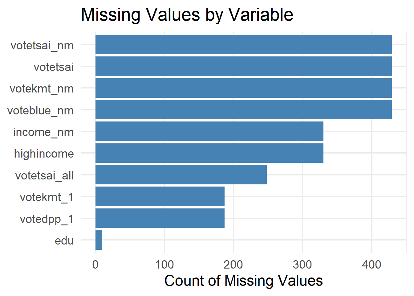
 NA's   :429                       NA's   :429      NA's   :248     
  Independence     Unification           sq           Taiwanese     
 Min.   :0.0000   Min.   :0.0000   Min.   :0.0000   Min.   :0.0000  
 1st Qu.:0.0000   1st Qu.:0.0000   1st Qu.:0.0000   1st Qu.:0.0000  
 Median :0.0000   Median :0.0000   Median :1.0000   Median :1.0000  
 Mean   :0.2888   Mean   :0.1225   Mean   :0.5172   Mean   :0.6272  
 3rd Qu.:1.0000   3rd Qu.:0.0000   3rd Qu.:1.0000   3rd Qu.:1.0000  
 Max.   :1.0000   Max.   :1.0000   Max.   :1.0000   Max.   :1.0000  
                                                                    
      edu            female        whitecollar       lowincome    
 Min.   :1.000   Min.   :0.0000   Min.   :0.0000   Min.   :1.000  
 1st Qu.:2.000   1st Qu.:0.0000   1st Qu.:0.0000   1st Qu.:4.000  
 Median :3.000   Median :0.0000   Median :1.0000   Median :5.000  
 Mean   :3.301   Mean   :0.4864   Mean   :0.5373   Mean   :4.343  
 3rd Qu.:5.000   3rd Qu.:1.0000   3rd Qu.:1.0000   3rd Qu.:5.000  
 Max.   :5.000   Max.   :1.0000   Max.   :1.0000   Max.   :5.000  
 NA's   :10                                                       
     income         income_nm           age              KMT        
 Min.   : 1.000   Min.   : 1.000   Min.   : 20.00   Min.   :0.0000  
 1st Qu.: 3.000   1st Qu.: 2.000   1st Qu.: 35.00   1st Qu.:0.0000  
 Median : 5.500   Median : 5.000   Median : 49.00   Median :0.0000  
 Mean   : 5.324   Mean   : 5.281   Mean   : 49.11   Mean   :0.2296  
 3rd Qu.: 7.000   3rd Qu.: 8.000   3rd Qu.: 61.00   3rd Qu.:0.0000  
 Max.   :10.000   Max.   :10.000   Max.   :100.00   Max.   :1.0000  
                  NA's   :330                                       
      DPP              npp             noparty            pfp         
 Min.   :0.0000   Min.   :0.00000   Min.   :0.0000   Min.   :0.00000  
 1st Qu.:0.0000   1st Qu.:0.00000   1st Qu.:0.0000   1st Qu.:0.00000  
 Median :0.0000   Median :0.00000   Median :0.0000   Median :0.00000  
 Mean   :0.3497   Mean   :0.02544   Mean   :0.3716   Mean   :0.01893  
 3rd Qu.:1.0000   3rd Qu.:0.00000   3rd Qu.:1.0000   3rd Qu.:0.00000  
 Max.   :1.0000   Max.   :1.00000   Max.   :1.0000   Max.   :1.00000  
                                                                      
     South            north        Minnan_father    Mainland_father 
 Min.   :0.0000   Min.   :0.0000   Min.   :0.0000   Min.   :0.0000  
 1st Qu.:0.0000   1st Qu.:0.0000   1st Qu.:0.0000   1st Qu.:0.0000  
 Median :0.0000   Median :0.0000   Median :1.0000   Median :0.0000  
 Mean   :0.4947   Mean   :0.4799   Mean   :0.7225   Mean   :0.1024  
 3rd Qu.:1.0000   3rd Qu.:1.0000   3rd Qu.:1.0000   3rd Qu.:0.0000  
 Max.   :1.0000   Max.   :1.0000   Max.   :1.0000   Max.   :1.0000  
                                                                    
   Econ_worse       Inequality      inequality5      econworse5   
 Min.   :0.0000   Min.   :0.0000   Min.   :1.000   Min.   :1.000  
 1st Qu.:0.0000   1st Qu.:1.0000   1st Qu.:4.000   1st Qu.:3.000  
 Median :1.0000   Median :1.0000   Median :5.000   Median :4.000  
 Mean   :0.5544   Mean   :0.9355   Mean   :4.495   Mean   :3.644  
 3rd Qu.:1.0000   3rd Qu.:1.0000   3rd Qu.:5.000   3rd Qu.:4.000  
 Max.   :1.0000   Max.   :1.0000   Max.   :5.000   Max.   :5.000  
                                                                  
 Govt_for_public     pubwelf5     Govt_dont_care     highincome    
 Min.   :0.0000   Min.   :1.000   Min.   :0.0000   Min.   :0.0000  
 1st Qu.:0.0000   1st Qu.:2.000   1st Qu.:0.0000   1st Qu.:0.0000  
 Median :0.0000   Median :3.000   Median :0.0000   Median :1.0000  
 Mean   :0.4249   Mean   :2.877   Mean   :0.4988   Mean   :0.5765  
 3rd Qu.:1.0000   3rd Qu.:4.000   3rd Qu.:1.0000   3rd Qu.:1.0000  
 Max.   :1.0000   Max.   :5.000   Max.   :1.0000   Max.   :1.0000  
                                                   NA's   :330     
    votekmt         votekmt_nm          Blue       Green      No_Party
 Min.   :0.0000   Min.   :0.0000   Min.   :0   Min.   :0   Min.   :0  
 1st Qu.:0.0000   1st Qu.:0.0000   1st Qu.:0   1st Qu.:0   1st Qu.:0  
 Median :0.0000   Median :0.0000   Median :0   Median :0   Median :0  
 Mean   :0.2053   Mean   :0.2752   Mean   :0   Mean   :0   Mean   :0  
 3rd Qu.:0.0000   3rd Qu.:1.0000   3rd Qu.:0   3rd Qu.:0   3rd Qu.:0  
 Max.   :1.0000   Max.   :1.0000   Max.   :0   Max.   :0   Max.   :0  
                  NA's   :429                                         
    voteblue       voteblue_nm       votedpp_1        votekmt_1     
 Min.   :0.0000   Min.   :0.0000   Min.   :0.0000   Min.   :0.0000  
 1st Qu.:0.0000   1st Qu.:0.0000   1st Qu.:0.0000   1st Qu.:0.0000  
 Median :0.0000   Median :0.0000   Median :1.0000   Median :0.0000  
 Mean   :0.2787   Mean   :0.3735   Mean   :0.5256   Mean   :0.2309  
 3rd Qu.:1.0000   3rd Qu.:1.0000   3rd Qu.:1.0000   3rd Qu.:0.0000  
 Max.   :1.0000   Max.   :1.0000   Max.   :1.0000   Max.   :1.0000  
                  NA's   :429      NA's   :187      NA's   :187     

# ----------------------------------------------------------------------------
# Q2. Missing data assessment
# ----------------------------------------------------------------------------

TEDS_2016 %>%
  summarise(across(everything(), ~sum(is.na(.)))) %>%
  pivot_longer(everything(), 
               names_to = "variable", 
               values_to = "n_missing") %>%
  filter(n_missing > 0) %>%
  arrange(desc(n_missing))

# A tibble: 10 × 2
   variable     n_missing
   <chr>            <int>
 1 votetsai           429
 2 votetsai_nm        429
 3 votekmt_nm         429
 4 voteblue_nm        429
 5 income_nm          330
 6 highincome         330
 7 votetsai_all       248
 8 votedpp_1          187
 9 votekmt_1          187
10 edu                 10

# Visualize missingness
TEDS_2016 %>%
  summarise(across(everything(), ~sum(is.na(.)))) %>%
  pivot_longer(everything(), 
               names_to = "variable", 
               values_to = "n_missing") %>%
  filter(n_missing > 0) %>%
  ggplot(aes(x = reorder(variable, n_missing), y = n_missing)) +
  geom_col(fill = "steelblue") +
  coord_flip() +
  labs(title = "Missing Values by Variable",
       x = NULL, y = "Count of Missing Values") +
  theme_minimal(base_size = 18)

# ----------------------------------------------------------------------------
# Q3. Variable recoding
# ----------------------------------------------------------------------------

teds <- TEDS_2016 %>%
  mutate(
    vote = factor(votetsai, 
                  levels = c(0, 1), 
                  labels = c("Other", "Tsai")),
    gender = factor(female, 
                    levels = c(0, 1), 
                    labels = c("Male", "Female")),
    Tondu = as.factor(Tondu),
    Party = as.factor(Party)
  ) %>%
  dplyr::select(vote, gender, age, edu, income, 
         Taiwanese, Econ_worse, Tondu, Party, DPP) %>%
  drop_na()

glimpse(teds)

Rows: 1,257
Columns: 10
$ vote       <fct> Tsai, Other, Tsai, Tsai, Tsai, Tsai, Tsai, Tsai, Other, Oth…
$ gender     <fct> Female, Male, Female, Male, Female, Female, Male, Female, F…
$ age        <dbl> 39, 63, 64, 75, 54, 64, 66, 25, 41, 57, 83, 43, 44, 34, 28,…
$ edu        <dbl> 5, 5, 2, 1, 5, 1, 1, 2, 5, 5, 1, 5, 5, 3, 3, 3, 3, 1, 5, 3,…
$ income     <dbl> 7.0, 8.0, 9.0, 1.0, 10.0, 2.0, 3.0, 5.5, 9.0, 1.0, 5.5, 5.0…
$ Taiwanese  <dbl> 0, 0, 1, 0, 1, 1, 1, 1, 1, 0, 0, 1, 1, 1, 0, 0, 0, 0, 0, 1,…
$ Econ_worse <dbl> 0, 1, 1, 1, 1, 1, 1, 0, 0, 1, 0, 1, 1, 0, 0, 0, 1, 0, 1, 0,…
$ Tondu      <fct> 5, 3, 4, 9, 6, 9, 5, 5, 5, 4, 9, 3, 5, 3, 3, 4, 1, 1, 4, 3,…
$ Party      <fct> 25, 3, 6, 25, 24, 25, 6, 5, 3, 3, 25, 23, 7, 3, 25, 2, 10, …
$ DPP        <dbl> 0, 0, 1, 0, 0, 0, 1, 1, 0, 0, 0, 0, 1, 0, 0, 0, 0, 0, 0, 1,…

# ----------------------------------------------------------------------------
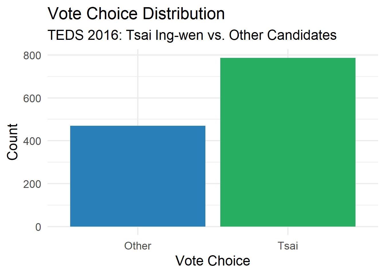
# Q4. Vote choice distribution
# ----------------------------------------------------------------------------

ggplot(teds, aes(x = vote, fill = vote)) +
  geom_bar() +
  scale_fill_manual(values = c("Other" = "#2980b9", "Tsai" = "#27ae60")) +
  labs(title = "Vote Choice Distribution",
       subtitle = "TEDS 2016: Tsai Ing-wen vs. Other Candidates",
       x = "Vote Choice", y = "Count") +
  theme_minimal(base_size = 18) +
  theme(legend.position = "none")

# ----------------------------------------------------------------------------
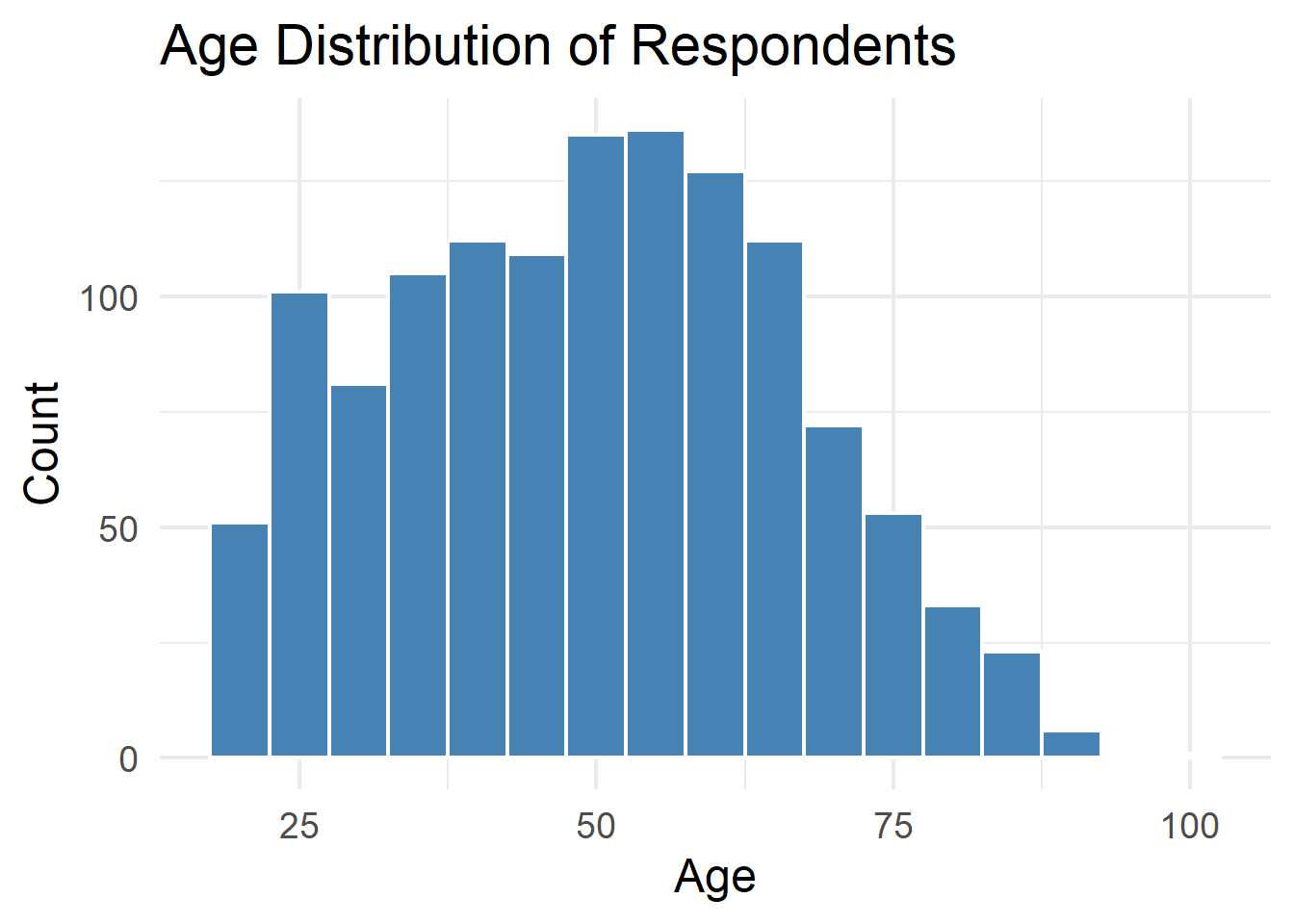
# Q5. Age distribution
# ----------------------------------------------------------------------------

ggplot(teds, aes(x = age)) +
  geom_histogram(binwidth = 5, fill = "steelblue", color = "white") +
  labs(title = "Age Distribution of Respondents",
       x = "Age", y = "Count") +
  theme_minimal(base_size = 18)

# ----------------------------------------------------------------------------
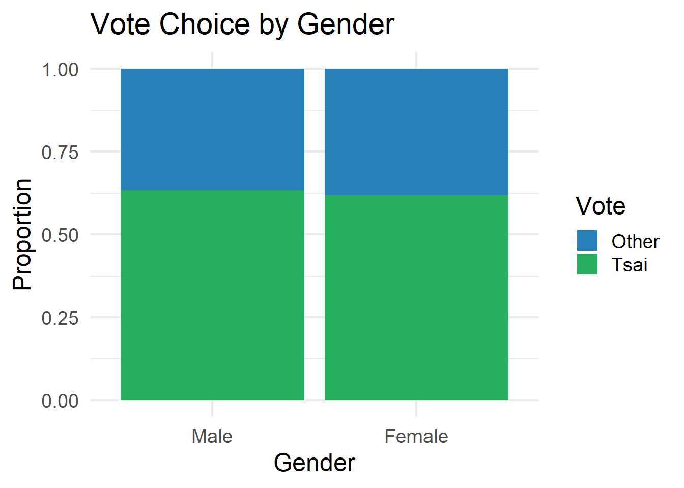
# Q6. Vote by gender
# ----------------------------------------------------------------------------

ggplot(teds, aes(x = gender, fill = vote)) +
  geom_bar(position = "fill") +
  scale_fill_manual(values = c("Other" = "#2980b9", "Tsai" = "#27ae60")) +
  labs(title = "Vote Choice by Gender",
       x = "Gender", y = "Proportion",
       fill = "Vote") +
  theme_minimal(base_size = 18)

# ----------------------------------------------------------------------------
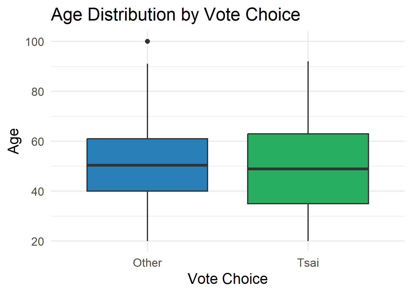
# Q7. Age by vote choice
# ----------------------------------------------------------------------------

ggplot(teds, aes(x = vote, y = age, fill = vote)) +
  geom_boxplot() +
  scale_fill_manual(values = c("Other" = "#2980b9", "Tsai" = "#27ae60")) +
  labs(title = "Age Distribution by Vote Choice",
       x = "Vote Choice", y = "Age") +
  theme_minimal(base_size = 18) +
  theme(legend.position = "none")

# ----------------------------------------------------------------------------
# Q8. Correlation matrix
# ----------------------------------------------------------------------------

teds %>%
  dplyr::select(age, edu, income, Taiwanese, Econ_worse, DPP) %>%
  cor(use = "complete.obs") %>%
  as.data.frame() %>%
  rownames_to_column("var1") %>%
  pivot_longer(-var1, names_to = "var2", values_to = "cor") %>%
  ggplot(aes(x = var1, y = var2, fill = cor)) +
  geom_tile() +
  geom_text(aes(label = round(cor, 2)), size = 6) +
  scale_fill_gradient2(low = "#e74c3c", mid = "white", high = "#2980b9",
                       midpoint = 0, limits = c(-1, 1)) +
  labs(title = "Correlation Matrix of Numeric Variables",
       x = NULL, y = NULL) +
  theme_minimal(base_size = 18) +
  theme(axis.text.x = element_text(angle = 45, hjust = 1))

# ----------------------------------------------------------------------------
# Q9. Pairs plot
# ----------------------------------------------------------------------------

teds %>%
  dplyr::select(age, edu, income, Taiwanese, Econ_worse, vote) %>%
  ggpairs(aes(color = vote, alpha = 0.5),
          upper = list(continuous = wrap("cor", size = 4)),
          lower = list(continuous = wrap("points", size = 0.5))) +
  scale_color_manual(values = c("Other" = "#2980b9", "Tsai" = "#27ae60")) +
  scale_fill_manual(values = c("Other" = "#2980b9", "Tsai" = "#27ae60")) +
  theme_minimal(base_size = 14)

Warning: No shared levels found between `names(values)` of the manual scale and the
data's colour values.

Warning: No shared levels found between `names(values)` of the manual scale and the
data's colour values.

Warning: No shared levels found between `names(values)` of the manual scale and the
data's fill values.

Warning: No shared levels found between `names(values)` of the manual scale and the
data's colour values.
No shared levels found between `names(values)` of the manual scale and the
data's colour values.

Warning: No shared levels found between `names(values)` of the manual scale and the
data's fill values.

Warning: No shared levels found between `names(values)` of the manual scale and the
data's colour values.
No shared levels found between `names(values)` of the manual scale and the
data's colour values.

Warning: No shared levels found between `names(values)` of the manual scale and the
data's fill values.

Warning: No shared levels found between `names(values)` of the manual scale and the
data's colour values.
No shared levels found between `names(values)` of the manual scale and the
data's colour values.

Warning: No shared levels found between `names(values)` of the manual scale and the
data's fill values.

Warning: No shared levels found between `names(values)` of the manual scale and the
data's colour values.
No shared levels found between `names(values)` of the manual scale and the
data's colour values.

Warning: No shared levels found between `names(values)` of the manual scale and the
data's fill values.

Warning: No shared levels found between `names(values)` of the manual scale and the
data's colour values.
No shared levels found between `names(values)` of the manual scale and the
data's colour values.

Warning: No shared levels found between `names(values)` of the manual scale and the
data's fill values.

Warning: No shared levels found between `names(values)` of the manual scale and the
data's colour values.
No shared levels found between `names(values)` of the manual scale and the
data's colour values.

Warning: No shared levels found between `names(values)` of the manual scale and the
data's fill values.

Warning: No shared levels found between `names(values)` of the manual scale and the
data's colour values.
No shared levels found between `names(values)` of the manual scale and the
data's colour values.

Warning: No shared levels found between `names(values)` of the manual scale and the
data's fill values.

Warning: No shared levels found between `names(values)` of the manual scale and the
data's colour values.
No shared levels found between `names(values)` of the manual scale and the
data's colour values.

Warning: No shared levels found between `names(values)` of the manual scale and the
data's fill values.
No shared levels found between `names(values)` of the manual scale and the
data's fill values.

Warning: No shared levels found between `names(values)` of the manual scale and the
data's colour values.
No shared levels found between `names(values)` of the manual scale and the
data's colour values.

Warning: No shared levels found between `names(values)` of the manual scale and the
data's fill values.

Warning: No shared levels found between `names(values)` of the manual scale and the
data's colour values.
No shared levels found between `names(values)` of the manual scale and the
data's colour values.

Warning: No shared levels found between `names(values)` of the manual scale and the
data's fill values.

Warning: No shared levels found between `names(values)` of the manual scale and the
data's colour values.
No shared levels found between `names(values)` of the manual scale and the
data's colour values.

Warning: No shared levels found between `names(values)` of the manual scale and the
data's fill values.
No shared levels found between `names(values)` of the manual scale and the
data's fill values.
No shared levels found between `names(values)` of the manual scale and the
data's fill values.

Warning: No shared levels found between `names(values)` of the manual scale and the
data's colour values.
No shared levels found between `names(values)` of the manual scale and the
data's colour values.

Warning: No shared levels found between `names(values)` of the manual scale and the
data's fill values.

Warning: No shared levels found between `names(values)` of the manual scale and the
data's colour values.
No shared levels found between `names(values)` of the manual scale and the
data's colour values.

Warning: No shared levels found between `names(values)` of the manual scale and the
data's fill values.
No shared levels found between `names(values)` of the manual scale and the
data's fill values.
No shared levels found between `names(values)` of the manual scale and the
data's fill values.
No shared levels found between `names(values)` of the manual scale and the
data's fill values.

Warning: No shared levels found between `names(values)` of the manual scale and the
data's colour values.
No shared levels found between `names(values)` of the manual scale and the
data's colour values.

`stat_bin()` using `bins = 30`. Pick better value `binwidth`.

Warning: No shared levels found between `names(values)` of the manual scale and the
data's colour values.

`stat_bin()` using `bins = 30`. Pick better value `binwidth`.

Warning: No shared levels found between `names(values)` of the manual scale and the
data's colour values.

`stat_bin()` using `bins = 30`. Pick better value `binwidth`.

Warning: No shared levels found between `names(values)` of the manual scale and the
data's colour values.

`stat_bin()` using `bins = 30`. Pick better value `binwidth`.

Warning: No shared levels found between `names(values)` of the manual scale and the
data's colour values.

`stat_bin()` using `bins = 30`. Pick better value `binwidth`.

Warning: No shared levels found between `names(values)` of the manual scale and the
data's colour values.
No shared levels found between `names(values)` of the manual scale and the
data's colour values.

# ============================================================================
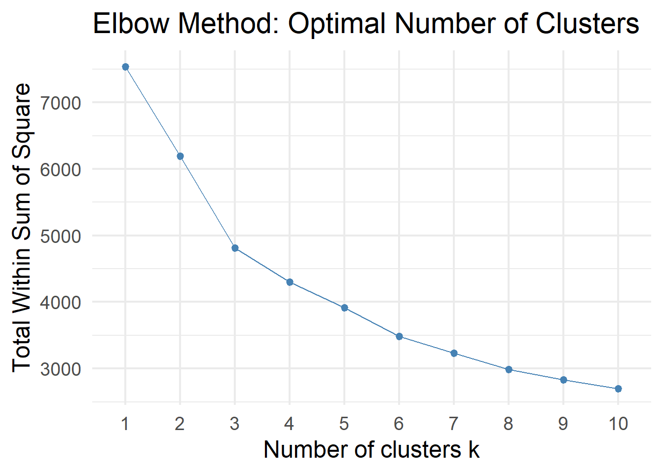
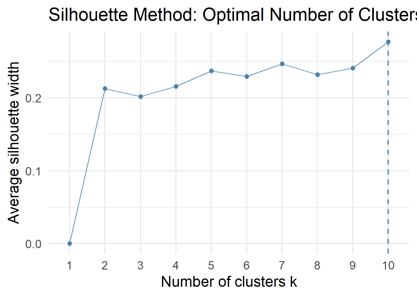
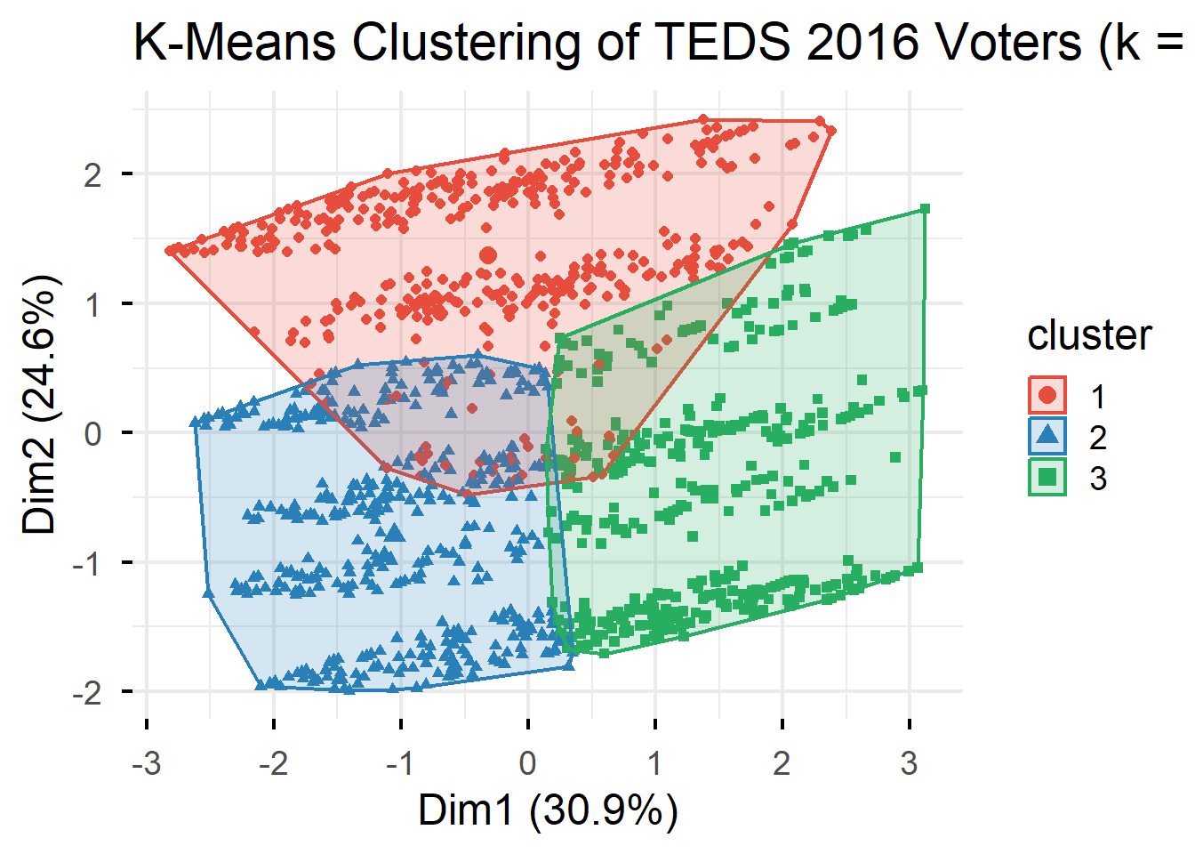
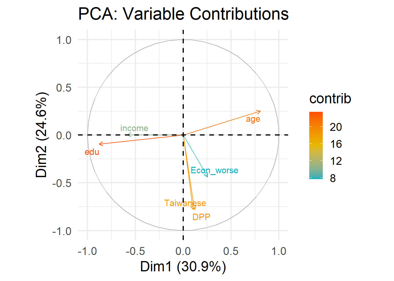
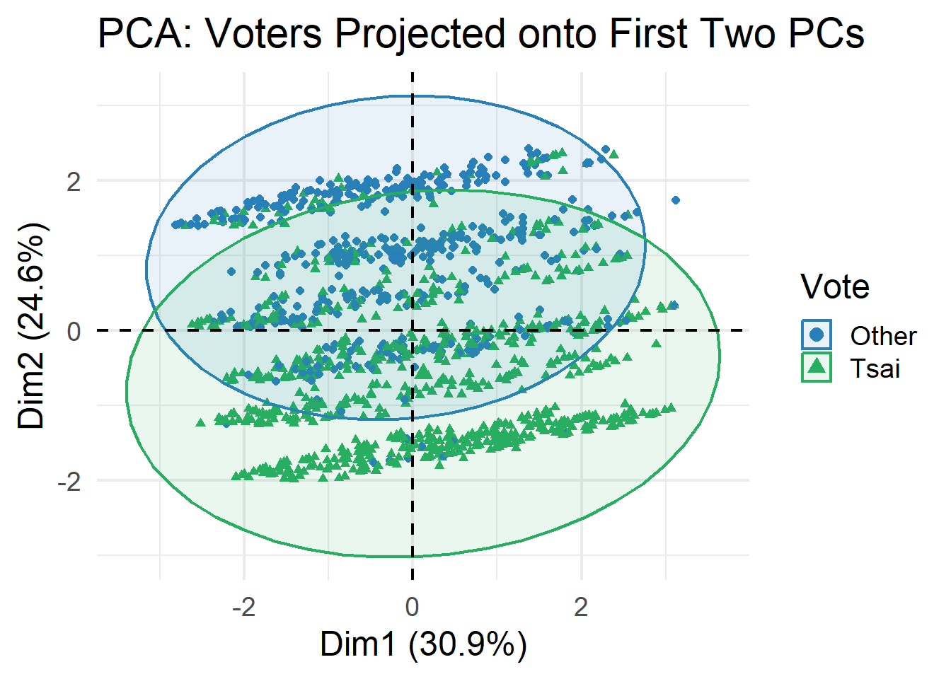
# PART II: UNSUPERVISED LEARNING
# ============================================================================

# ----------------------------------------------------------------------------
# Prepare data for clustering
# ----------------------------------------------------------------------------

teds_numeric <- teds %>%
  dplyr::select(age, edu, income, Taiwanese, Econ_worse, DPP) %>%
  scale() %>%
  as.data.frame()

head(teds_numeric)

         age        edu     income Taiwanese Econ_worse        DPP
1 -0.6442434  1.1180557  0.5890616 -1.352636 -1.1612317 -0.8507077
2  0.7997042  1.1180557  0.9453043 -1.352636  0.8604695 -0.8507077
3  0.8598687 -0.8791912  1.3015470  0.738709  0.8604695  1.1745567
4  1.5216780 -1.5449401 -1.5483945 -1.352636  0.8604695 -0.8507077
5  0.2582239  1.1180557  1.6577897  0.738709  0.8604695 -0.8507077
6  0.8598687 -1.5449401 -1.1921518  0.738709  0.8604695 -0.8507077

# ----------------------------------------------------------------------------
# Q10. Choosing k: Elbow method
# ----------------------------------------------------------------------------

fviz_nbclust(teds_numeric, kmeans, method = "wss", k.max = 10) +
  labs(title = "Elbow Method: Optimal Number of Clusters") +
  theme_minimal(base_size = 18)

# Silhouette method
fviz_nbclust(teds_numeric, kmeans, method = "silhouette", k.max = 10) +
  labs(title = "Silhouette Method: Optimal Number of Clusters") +
  theme_minimal(base_size = 18)

# ----------------------------------------------------------------------------
# Q11. K-Means clustering
# ----------------------------------------------------------------------------

set.seed(6323)
km_result <- kmeans(teds_numeric, centers = 3, nstart = 25)

table(km_result$cluster)

  1   2   3 
400 442 415 

round(km_result$centers, 2)

    age   edu income Taiwanese Econ_worse   DPP
1  0.11  0.17   0.15     -1.35      -0.26 -0.62
2 -0.80  0.75   0.37      0.69      -0.05  0.24
3  0.74 -0.96  -0.54      0.57       0.31  0.35

# Visualize clusters
fviz_cluster(km_result, data = teds_numeric,
             geom = "point", 
             ellipse.type = "convex",
             palette = c("#e74c3c", "#2980b9", "#27ae60"),
             ggtheme = theme_minimal(base_size = 18)) +
  labs(title = "K-Means Clustering of TEDS 2016 Voters (k = 3)")

# ----------------------------------------------------------------------------
# Q12. Cluster profiling
# ----------------------------------------------------------------------------

teds$cluster <- as.factor(km_result$cluster)

teds %>%
  group_by(cluster) %>%
  summarise(
    n = n(),
    mean_age = round(mean(age), 1),
    mean_edu = round(mean(edu), 1),
    mean_income = round(mean(income), 1),
    pct_Taiwanese = round(mean(Taiwanese) * 100, 1),
    pct_Econ_worse = round(mean(Econ_worse) * 100, 1),
    mean_DPP = round(mean(DPP), 2),
    pct_Tsai = round(mean(vote == "Tsai") * 100, 1)
  )

# A tibble: 3 × 9
  cluster     n mean_age mean_edu mean_income pct_Taiwanese pct_Econ_worse
  <fct>   <int>    <dbl>    <dbl>       <dbl>         <dbl>          <dbl>
1 1         400     51.6      3.6         5.8           0             44.5
2 2         442     36.4      4.4         6.4          97.5           54.8
3 3         415     62        1.9         3.8          92             72.8
# ℹ 2 more variables: mean_DPP <dbl>, pct_Tsai <dbl>

# ----------------------------------------------------------------------------
# Q13. Clusters vs. vote choice
# ----------------------------------------------------------------------------

ggplot(teds, aes(x = cluster, fill = vote)) +
  geom_bar(position = "fill") +
  scale_fill_manual(values = c("Other" = "#2980b9", "Tsai" = "#27ae60")) +
  labs(title = "Vote Choice Distribution by Cluster",
       x = "Cluster", y = "Proportion",
       fill = "Vote") +
  theme_minimal(base_size = 18)

# ----------------------------------------------------------------------------
# Q14. Principal Component Analysis
# ----------------------------------------------------------------------------

pca_result <- prcomp(teds_numeric, scale. = TRUE)
summary(pca_result)

Importance of components:
                          PC1    PC2    PC3    PC4    PC5    PC6
Standard deviation     1.3621 1.2153 0.9492 0.9141 0.7843 0.5623
Proportion of Variance 0.3092 0.2461 0.1502 0.1393 0.1025 0.0527
Cumulative Proportion  0.3092 0.5554 0.7055 0.8448 0.9473 1.0000

# Scree plot
fviz_eig(pca_result, addlabels = TRUE) +
  labs(title = "Scree Plot: Variance Explained by Each PC") +
  theme_minimal(base_size = 18)

# ----------------------------------------------------------------------------
# Q15. PCA variable contributions
# ----------------------------------------------------------------------------

fviz_pca_var(pca_result, 
             col.var = "contrib",
             gradient.cols = c("#00AFBB", "#E7B800", "#FC4E07"),
             repel = TRUE) +
  labs(title = "PCA: Variable Contributions") +
  theme_minimal(base_size = 18)

# PCA individuals by vote
fviz_pca_ind(pca_result,
             geom = "point",
             col.ind = teds$vote,
             palette = c("#2980b9", "#27ae60"),
             addEllipses = TRUE,
             legend.title = "Vote") +
  labs(title = "PCA: Voters Projected onto First Two PCs") +
  theme_minimal(base_size = 18)

Ignoring unknown labels:
• linetype : "Vote"

# ============================================================================
# PART III: SUPERVISED LEARNING
# ============================================================================

# ----------------------------------------------------------------------------
# Q16. Train-test split
# ----------------------------------------------------------------------------

set.seed(6323)

train_index <- createDataPartition(teds$vote, p = 0.7, list = FALSE)
train_data <- teds[train_index, ] %>% dplyr::select(-cluster)
test_data  <- teds[-train_index, ] %>% dplyr::select(-cluster)

cat("Training set:", nrow(train_data), "observations\n")

Training set: 880 observations

cat("Test set:", nrow(test_data), "observations\n")

Test set: 377 observations

prop.table(table(train_data$vote))

    Other      Tsai 
0.3738636 0.6261364 

# ----------------------------------------------------------------------------
# Q17. Logistic regression
# ----------------------------------------------------------------------------

logit_model <- glm(vote ~ age + gender + edu + income + 
                     Taiwanese + Econ_worse + DPP,
                   data = train_data, 
                   family = binomial)

summary(logit_model)

Call:
glm(formula = vote ~ age + gender + edu + income + Taiwanese + 
    Econ_worse + DPP, family = binomial, data = train_data)

Coefficients:
              Estimate Std. Error z value Pr(>|z|)    
(Intercept)   0.361867   0.642494   0.563  0.57328    
age          -0.016301   0.007529  -2.165  0.03038 *  
genderFemale -0.349449   0.198576  -1.760  0.07845 .  
edu          -0.236898   0.089984  -2.633  0.00847 ** 
income       -0.017889   0.036531  -0.490  0.62435    
Taiwanese     1.483033   0.200581   7.394 1.43e-13 ***
Econ_worse    0.340277   0.193553   1.758  0.07874 .  
DPP           3.620753   0.315087  11.491  < 2e-16 ***
---
Signif. codes:  0 '***' 0.001 '**' 0.01 '*' 0.05 '.' 0.1 ' ' 1

(Dispersion parameter for binomial family taken to be 1)

    Null deviance: 1163.32  on 879  degrees of freedom
Residual deviance:  682.87  on 872  degrees of freedom
AIC: 698.87

Number of Fisher Scoring iterations: 6

# Evaluation
logit_probs <- predict(logit_model, newdata = test_data, type = "response")
logit_pred <- ifelse(logit_probs > 0.5, "Tsai", "Other")
logit_pred <- factor(logit_pred, levels = c("Other", "Tsai"))

confusionMatrix(logit_pred, test_data$vote)

Confusion Matrix and Statistics

          Reference
Prediction Other Tsai
     Other   104   40
     Tsai     37  196
                                          
               Accuracy : 0.7958          
                 95% CI : (0.7515, 0.8353)
    No Information Rate : 0.626           
    P-Value [Acc > NIR] : 8.186e-13       
                                          
                  Kappa : 0.5657          
                                          
 Mcnemar's Test P-Value : 0.8197          
                                          
            Sensitivity : 0.7376          
            Specificity : 0.8305          
         Pos Pred Value : 0.7222          
         Neg Pred Value : 0.8412          
             Prevalence : 0.3740          
         Detection Rate : 0.2759          
   Detection Prevalence : 0.3820          
      Balanced Accuracy : 0.7840          
                                          
       'Positive' Class : Other           
                                          

# ----------------------------------------------------------------------------
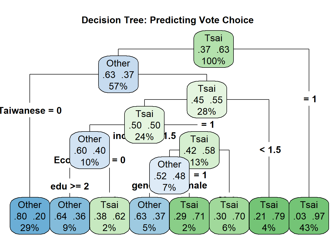
# Q18. Decision tree
# ----------------------------------------------------------------------------

tree_model <- rpart(vote ~ age + gender + edu + income + 
                      Taiwanese + Econ_worse + DPP,
                    data = train_data,
                    method = "class")

rpart.plot(tree_model, 
           type = 4, 
           extra = 104,
           main = "Decision Tree: Predicting Vote Choice",
           box.palette = "BuGn",
           cex = 1.2)

# Evaluation
tree_pred <- predict(tree_model, newdata = test_data, type = "class")
confusionMatrix(tree_pred, test_data$vote)

Confusion Matrix and Statistics

          Reference
Prediction Other Tsai
     Other   118   54
     Tsai     23  182
                                          
               Accuracy : 0.7958          
                 95% CI : (0.7515, 0.8353)
    No Information Rate : 0.626           
    P-Value [Acc > NIR] : 8.186e-13       
                                          
                  Kappa : 0.5823          
                                          
 Mcnemar's Test P-Value : 0.0006289       
                                          
            Sensitivity : 0.8369          
            Specificity : 0.7712          
         Pos Pred Value : 0.6860          
         Neg Pred Value : 0.8878          
             Prevalence : 0.3740          
         Detection Rate : 0.3130          
   Detection Prevalence : 0.4562          
      Balanced Accuracy : 0.8040          
                                          
       'Positive' Class : Other           
                                          

# ----------------------------------------------------------------------------
# Q19. Random forest
# ----------------------------------------------------------------------------

set.seed(6323)

rf_model <- randomForest(vote ~ age + gender + edu + income + 
                           Taiwanese + Econ_worse + DPP,
                         data = train_data,
                         ntree = 500,
                         importance = TRUE)

print(rf_model)

Call:
 randomForest(formula = vote ~ age + gender + edu + income + Taiwanese +      Econ_worse + DPP, data = train_data, ntree = 500, importance = TRUE) 
               Type of random forest: classification
                     Number of trees: 500
No. of variables tried at each split: 2

        OOB estimate of  error rate: 19.77%
Confusion matrix:
      Other Tsai class.error
Other   245   84   0.2553191
Tsai     90  461   0.1633394

# Evaluation
rf_pred <- predict(rf_model, newdata = test_data)
confusionMatrix(rf_pred, test_data$vote)

Confusion Matrix and Statistics

          Reference
Prediction Other Tsai
     Other   111   40
     Tsai     30  196
                                          
               Accuracy : 0.8143          
                 95% CI : (0.7713, 0.8523)
    No Information Rate : 0.626           
    P-Value [Acc > NIR] : 1.408e-15       
                                          
                  Kappa : 0.609           
                                          
 Mcnemar's Test P-Value : 0.2821          
                                          
            Sensitivity : 0.7872          
            Specificity : 0.8305          
         Pos Pred Value : 0.7351          
         Neg Pred Value : 0.8673          
             Prevalence : 0.3740          
         Detection Rate : 0.2944          
   Detection Prevalence : 0.4005          
      Balanced Accuracy : 0.8089          
                                          
       'Positive' Class : Other           
                                          

# ----------------------------------------------------------------------------
# Q20. Variable importance
# ----------------------------------------------------------------------------

importance_df <- as.data.frame(importance(rf_model)) %>%
  rownames_to_column("variable") %>%
  arrange(desc(MeanDecreaseGini))

ggplot(importance_df, aes(x = reorder(variable, MeanDecreaseGini), 
                           y = MeanDecreaseGini)) +
  geom_col(fill = "steelblue") +
  coord_flip() +
  labs(title = "Random Forest: Variable Importance",
       subtitle = "Mean Decrease in Gini Index",
       x = NULL, y = "Importance") +
  theme_minimal(base_size = 18)

# ----------------------------------------------------------------------------
# Q21. Model comparison
# ----------------------------------------------------------------------------

results <- tibble(
  Model = c("Logistic Regression", "Decision Tree", "Random Forest"),
  Accuracy = c(
    confusionMatrix(logit_pred, test_data$vote)$overall["Accuracy"],
    confusionMatrix(tree_pred, test_data$vote)$overall["Accuracy"],
    confusionMatrix(rf_pred, test_data$vote)$overall["Accuracy"]
  )
)

results %>% arrange(desc(Accuracy))

# A tibble: 3 × 2
  Model               Accuracy
  <chr>                  <dbl>
1 Random Forest          0.814
2 Logistic Regression    0.796
3 Decision Tree          0.796

# Comparison plot
ggplot(results, aes(x = reorder(Model, Accuracy), y = Accuracy, fill = Model)) +
  geom_col(width = 0.6) +
  geom_text(aes(label = paste0(round(Accuracy * 100, 1), "%")), 
            hjust = -0.1, size = 7) +
  coord_flip() +
  scale_fill_manual(values = c("#e74c3c", "#2980b9", "#27ae60")) +
  scale_y_continuous(limits = c(0, 1), labels = scales::percent) +
  labs(title = "Model Comparison: Prediction Accuracy",
       x = NULL, y = "Accuracy") +
  theme_minimal(base_size = 18) +
  theme(legend.position = "none")

TEDS2016 Dataset for Multiple Regression Models

#3. Use the TEDS2016 dataset to run a multiple regression model. Access the data set using the following codes: 
library(haven)

TEDS_2016 <- read_stata("https://github.com/datageneration/home/blob/master/DataProgramming/data/TEDS_2016.dta?raw=true")

names(TEDS_2016)

 [1] "District"        "Sex"             "Age"             "Edu"            
 [5] "Arear"           "Career"          "Career8"         "Ethnic"         
 [9] "Party"           "PartyID"         "Tondu"           "Tondu3"         
[13] "nI2"             "votetsai"        "green"           "votetsai_nm"    
[17] "votetsai_all"    "Independence"    "Unification"     "sq"             
[21] "Taiwanese"       "edu"             "female"          "whitecollar"    
[25] "lowincome"       "income"          "income_nm"       "age"            
[29] "KMT"             "DPP"             "npp"             "noparty"        
[33] "pfp"             "South"           "north"           "Minnan_father"  
[37] "Mainland_father" "Econ_worse"      "Inequality"      "inequality5"    
[41] "econworse5"      "Govt_for_public" "pubwelf5"        "Govt_dont_care" 
[45] "highincome"      "votekmt"         "votekmt_nm"      "Blue"           
[49] "Green"           "No_Party"        "voteblue"        "voteblue_nm"    
[53] "votedpp_1"       "votekmt_1"      

lm.fit <- lm(PartyID ~ Age + Edu + income, data = TEDS_2016)
summary(lm.fit)

Call:
lm(formula = PartyID ~ Age + Edu + income, data = TEDS_2016)

Residuals:
   Min     1Q Median     3Q    Max 
-5.038 -2.963 -2.121  4.135  6.622 

Coefficients:
            Estimate Std. Error t value Pr(>|t|)    
(Intercept)  7.00058    0.42994  16.283  < 2e-16 ***
Age         -0.28172    0.07176  -3.926 9.00e-05 ***
Edu         -0.29039    0.06906  -4.205 2.75e-05 ***
income      -0.10909    0.03301  -3.304 0.000972 ***
---
Signif. codes:  0 '***' 0.001 '**' 0.01 '*' 0.05 '.' 0.1 ' ' 1

Residual standard error: 3.511 on 1686 degrees of freedom
Multiple R-squared:  0.02327,   Adjusted R-squared:  0.02153 
F-statistic: 13.39 on 3 and 1686 DF,  p-value: 1.233e-08

library(car)

Loading required package: carData

Warning: package 'carData' was built under R version 4.5.2

Attaching package: 'car'

The following object is masked from 'package:dplyr':

    recode

The following object is masked from 'package:purrr':

    some

vif(lm.fit)

     Age      Edu   income 
1.455295 1.568808 1.118965 

lm.fit1 <- update(lm.fit, ~ . - Age)
summary(lm.fit1)

Call:
lm(formula = PartyID ~ Edu + income, data = TEDS_2016)

Residuals:
   Min     1Q Median     3Q    Max 
-4.326 -2.992 -2.100  4.158  5.320 

Coefficients:
            Estimate Std. Error t value Pr(>|t|)    
(Intercept)  5.57907    0.23277  23.969  < 2e-16 ***
Edu         -0.14519    0.05857  -2.479  0.01328 *  
income      -0.10765    0.03315  -3.247  0.00119 ** 
---
Signif. codes:  0 '***' 0.001 '**' 0.01 '*' 0.05 '.' 0.1 ' ' 1

Residual standard error: 3.526 on 1687 degrees of freedom
Multiple R-squared:  0.01434,   Adjusted R-squared:  0.01317 
F-statistic: 12.27 on 2 and 1687 DF,  p-value: 5.125e-06

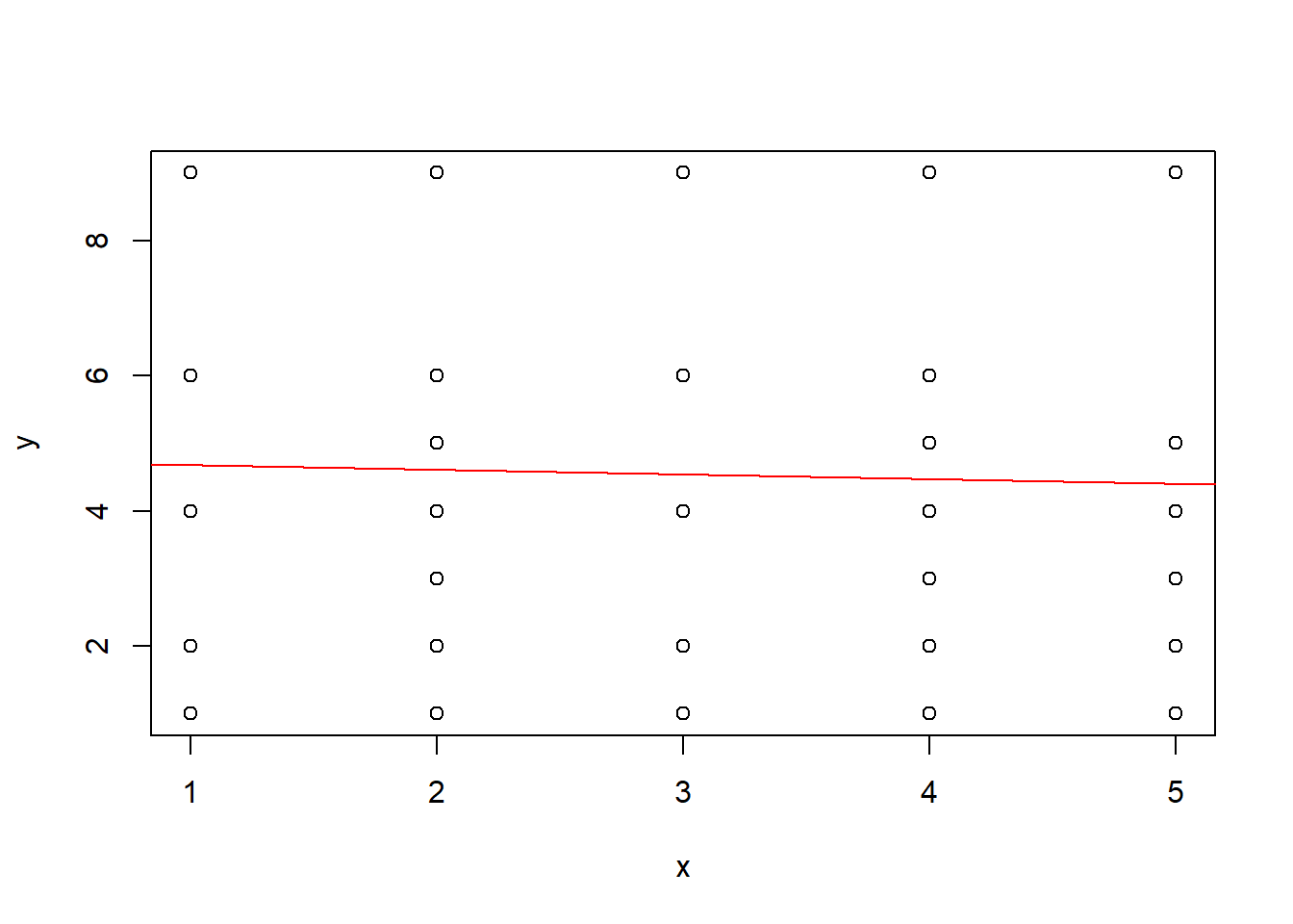
#4. Write a function called regplot to plot a regression line 
regplot=function(x,y){ 
  fit=lm(y~x) 
  plot(x,y) 
  abline(fit,col="red") 
} 

#5. Run a regplot on the dependent variable using Age, Education, Income
regplot(TEDS_2016$Age, TEDS_2016$PartyID)

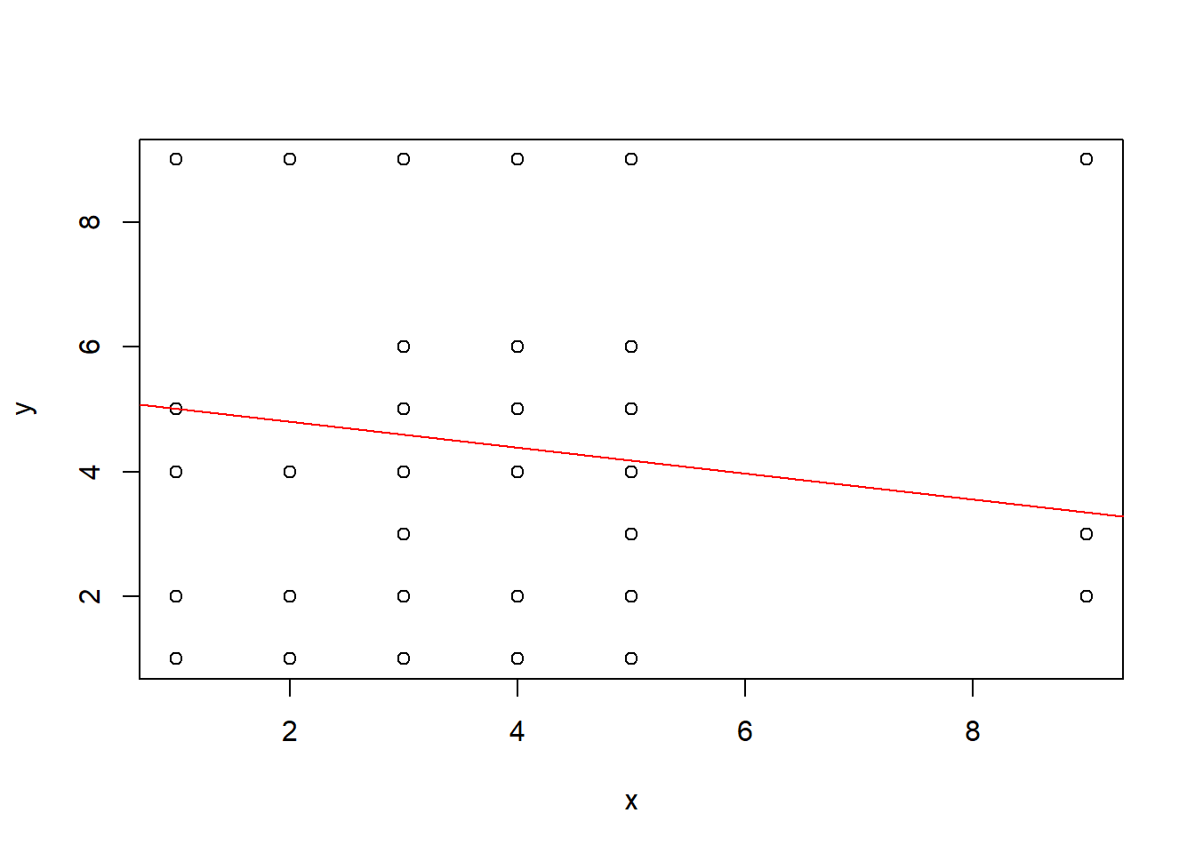
regplot(TEDS_2016$Edu, TEDS_2016$PartyID)

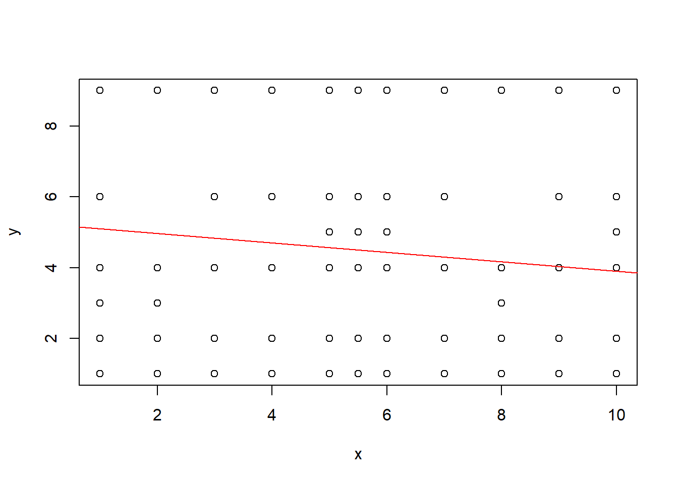
regplot(TEDS_2016$income, TEDS_2016$PartyID)

The problem with these plots is that the dependent variables for the regplots only have four categories rather than it being continuous. Therefore, the points appear to be in stacked horizontal levels, which indicates that the regression lines are not appropriate to model their relationships.

In order to improve the predictions of the dependent variables, a model designed for two or more categorical DV’s such as a logistic regression can help predict discrete results for the multiple regression models.