Assignment 1: Brush Up R and Quarto

Lab01:

R Programming Basic Commands

Create object using the assignment operator (<-, =)

x <- c(1,3,2,5)
x

[1] 1 3 2 5

x = c(1,6,2)
x

[1] 1 6 2

y = c(1,4,3)

Using function

length(x)  # What does length() do?

[1] 3

length(y)

[1] 3

Using +, -, *, /,^ operators

x+y

[1]  2 10  5

ls() # List objects in the environment

[1] "x" "y"

rm(x,y) # Remove objects
ls()

character(0)

rm(list=ls()) # Danger! What does this do?  Not recommended!

Matrix operations

?matrix

starting httpd help server ... done

x=matrix(data=c(1,2,3,4), nrow=2, ncol=2) # Create a 2x2 matrix object
x

     [,1] [,2]
[1,]    1    3
[2,]    2    4

x=matrix(c(1,2,3,4),2,2)
matrix(c(1,2,3,4),2,2,byrow=T) # What about byrow=F?

     [,1] [,2]
[1,]    1    2
[2,]    3    4

sqrt(x) # What does x look like?

         [,1]     [,2]
[1,] 1.000000 1.732051
[2,] 1.414214 2.000000

     [,1] [,2]
[1,]    1    3
[2,]    2    4

x^2

     [,1] [,2]
[1,]    1    9
[2,]    4   16

x=rnorm(50) # Generate a vector of 50 numbers using the rnorm() function

y=x+rnorm(50,mean=50,sd=.1) # What does rnorm(50,mean=50,sd=.1) generate?

cor(x,y) # Correlation of x and y

[1] 0.9915586

set.seed(1303) # Set the seed for Random Number Generator (RNG) to generate values that are reproducible.
rnorm(50)

 [1] -1.1439763145  1.3421293656  2.1853904757  0.5363925179  0.0631929665
 [6]  0.5022344825 -0.0004167247  0.5658198405 -0.5725226890 -1.1102250073
[11] -0.0486871234 -0.6956562176  0.8289174803  0.2066528551 -0.2356745091
[16] -0.5563104914 -0.3647543571  0.8623550343 -0.6307715354  0.3136021252
[21] -0.9314953177  0.8238676185  0.5233707021  0.7069214120  0.4202043256
[26] -0.2690521547 -1.5103172999 -0.6902124766 -0.1434719524 -1.0135274099
[31]  1.5732737361  0.0127465055  0.8726470499  0.4220661905 -0.0188157917
[36]  2.6157489689 -0.6931401748 -0.2663217810 -0.7206364412  1.3677342065
[41]  0.2640073322  0.6321868074 -1.3306509858  0.0268888182  1.0406363208
[46]  1.3120237985 -0.0300020767 -0.2500257125  0.0234144857  1.6598706557

set.seed(3) # Try different seeds?
y=rnorm(100)

Simple descriptive statistics (base)

mean(y)

[1] 0.01103557

var(y)

[1] 0.7328675

sqrt(var(y))

[1] 0.8560768

sd(y)

[1] 0.8560768

Visualization using R Graphics (without packages)

x=rnorm(100)
y=rnorm(100)
plot(x,y)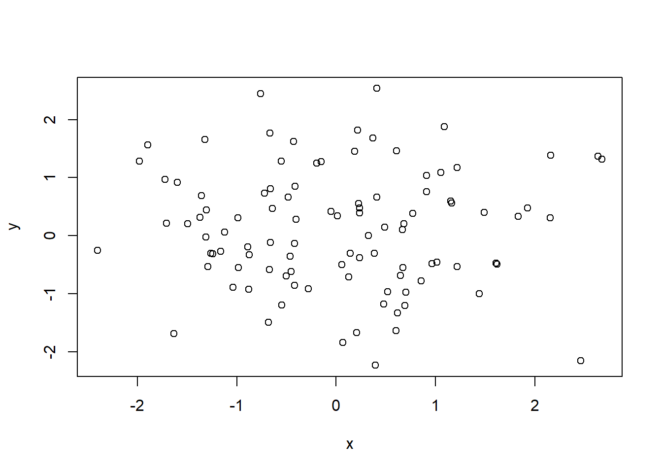

plot(x,y, pch=20, col = "firebrick") # Scatterplot for two numeric variables by default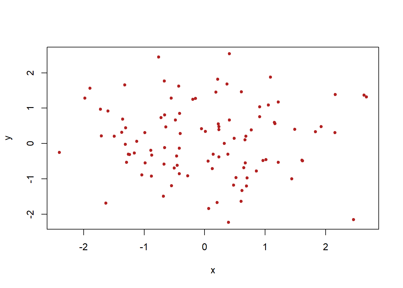

plot(x,y, pch=20, col = "steelblue",xlab="this is the x-axis",ylab="this is the y-axis",main="Plot of X vs Y") # Add labels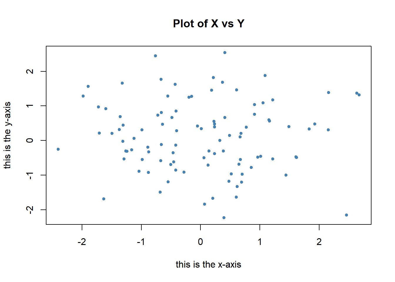

pdf("Figure01.pdf") # Save as pdf, add a path or it will be stored on the project directory
plot(x,y,pch=20, col="forestgreen") # Try different colors?
dev.off() # Close the file using the dev.off function

png 
  2

x=seq(1,10) # Same as x=c(1:10)
x

 [1]  1  2  3  4  5  6  7  8  9 10

x=1:10
x

 [1]  1  2  3  4  5  6  7  8  9 10

x=seq(-pi,pi,length=50)
y=x

Lab02:

R Programming Basic Commands

(Adapted from ISLR Chapter 3 Lab: Introduction to R)

Indexing Data using []

A=matrix(1:16,4,4)
A

     [,1] [,2] [,3] [,4]
[1,]    1    5    9   13
[2,]    2    6   10   14
[3,]    3    7   11   15
[4,]    4    8   12   16

A[2,3]

[1] 10

A[c(1,3),c(2,4)]

     [,1] [,2]
[1,]    5   13
[2,]    7   15

A[1:3,2:4]

     [,1] [,2] [,3]
[1,]    5    9   13
[2,]    6   10   14
[3,]    7   11   15

A[1:2,]

     [,1] [,2] [,3] [,4]
[1,]    1    5    9   13
[2,]    2    6   10   14

A[,1:2]

     [,1] [,2]
[1,]    1    5
[2,]    2    6
[3,]    3    7
[4,]    4    8

A[1,]

[1]  1  5  9 13

A[-c(1,3),] # What does -c() do?

     [,1] [,2] [,3] [,4]
[1,]    2    6   10   14
[2,]    4    8   12   16

A[-c(1,3),-c(1,3,4)]

[1] 6 8

dim(A) # Dimensions

[1] 4 4

Loading Data from GitHub (remote)

Auto=read.table("https://raw.githubusercontent.com/datageneration/knowledgemining/master/data/Auto.data")
Auto=read.table("https://raw.githubusercontent.com/datageneration/knowledgemining/master/data/Auto.data",header=T,na.strings="?") 
Auto=read.csv("https://raw.githubusercontent.com/datageneration/knowledgemining/master/data/Auto.csv") # read csv file
# Which function reads data faster?

# Try using this simple method
# time1 = proc.time()
# Auto=read.csv("https://raw.githubusercontent.com/datageneration/knowledgemining/master/data/Auto.csv",header=T,na.strings="?")
# proc.time()-time1

# Check on data
dim(Auto)

[1] 397   9

Auto[1:4,] # select rows

  mpg cylinders displacement horsepower weight acceleration year origin
1  18         8          307        130   3504         12.0   70      1
2  15         8          350        165   3693         11.5   70      1
3  18         8          318        150   3436         11.0   70      1
4  16         8          304        150   3433         12.0   70      1
                       name
1 chevrolet chevelle malibu
2         buick skylark 320
3        plymouth satellite
4             amc rebel sst

Auto=na.omit(Auto)
dim(Auto) # Notice the difference?

[1] 397   9

names(Auto)

[1] "mpg"          "cylinders"    "displacement" "horsepower"   "weight"      
[6] "acceleration" "year"         "origin"       "name"

Load data from ISLR website

Auto=read.table("https://www.statlearning.com/s/Auto.data",header=T,na.strings="?")
dim(Auto)

[1] 397   9

Additional Graphical and Numerical Summaries

# plot(cylinders, mpg)
plot(Auto$cylinders, Auto$mpg)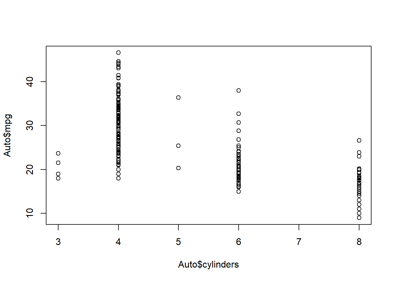

attach(Auto)
plot(cylinders, mpg)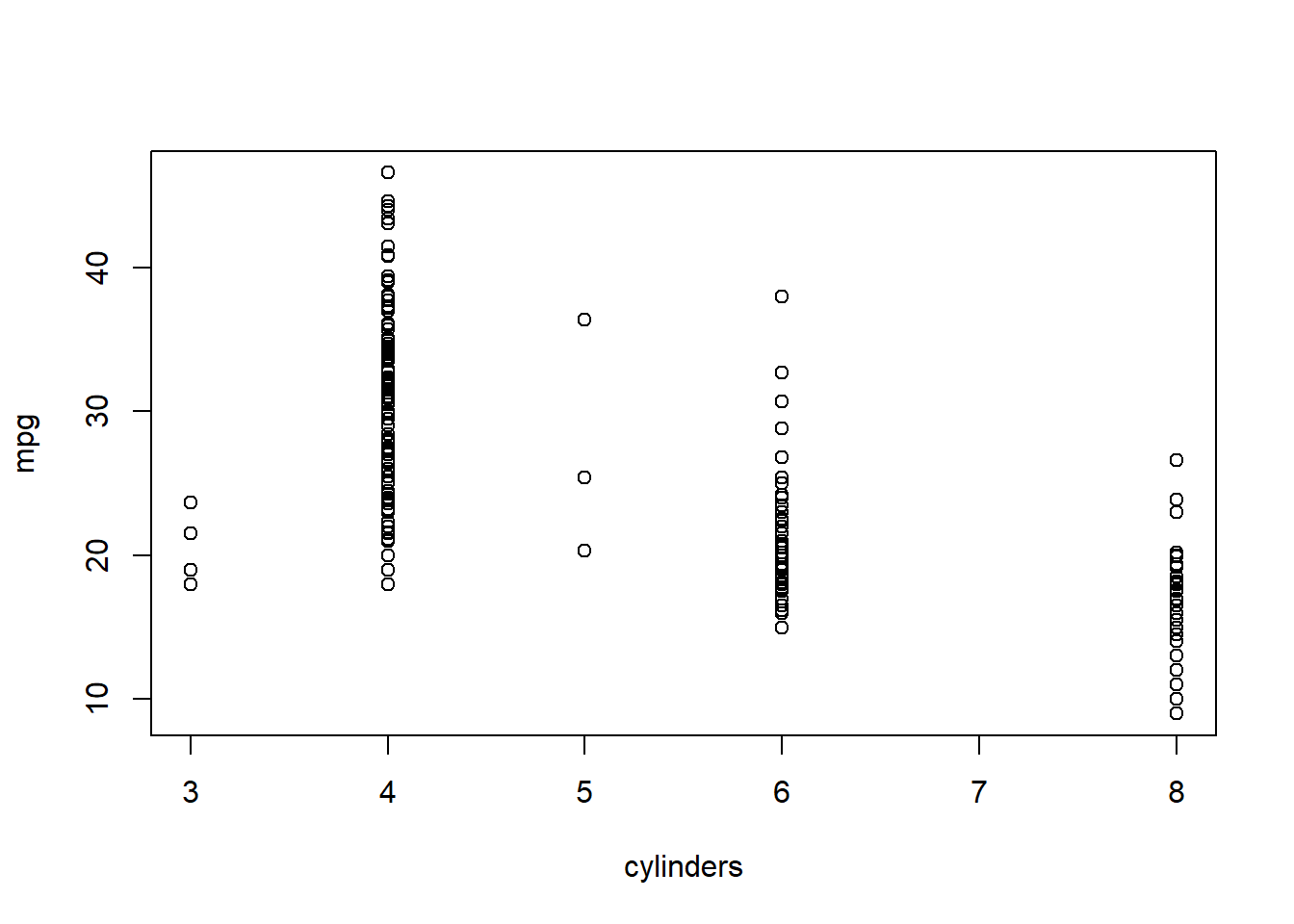

cylinders=as.factor(cylinders)
plot(cylinders, mpg)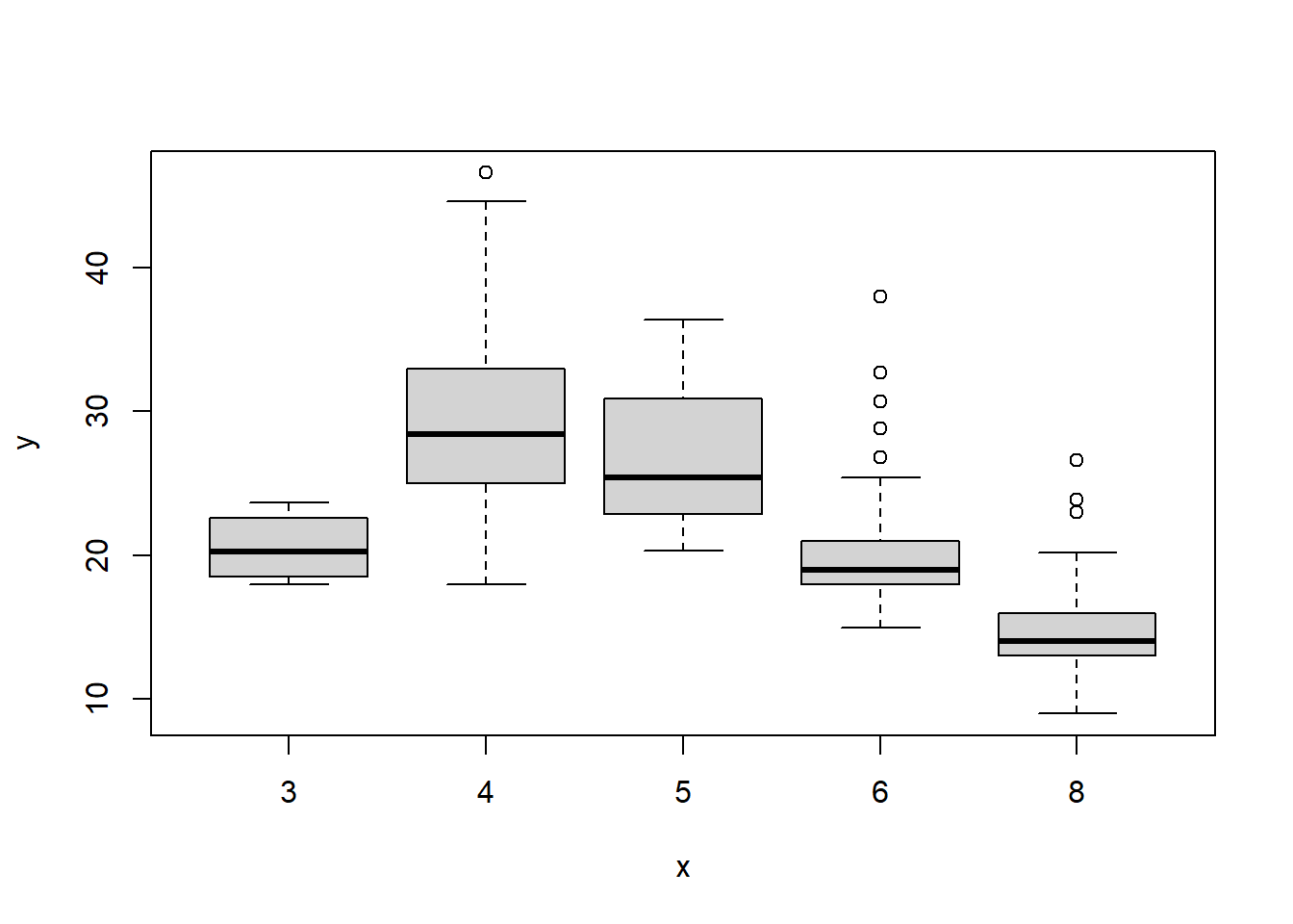

plot(cylinders, mpg, col="red")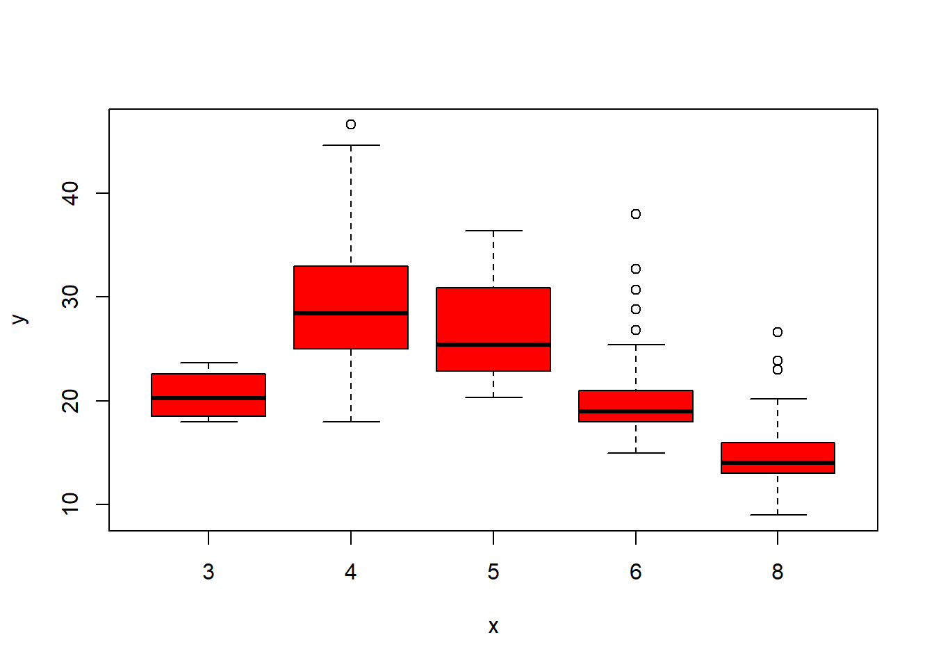

plot(cylinders, mpg, col="red", varwidth=T)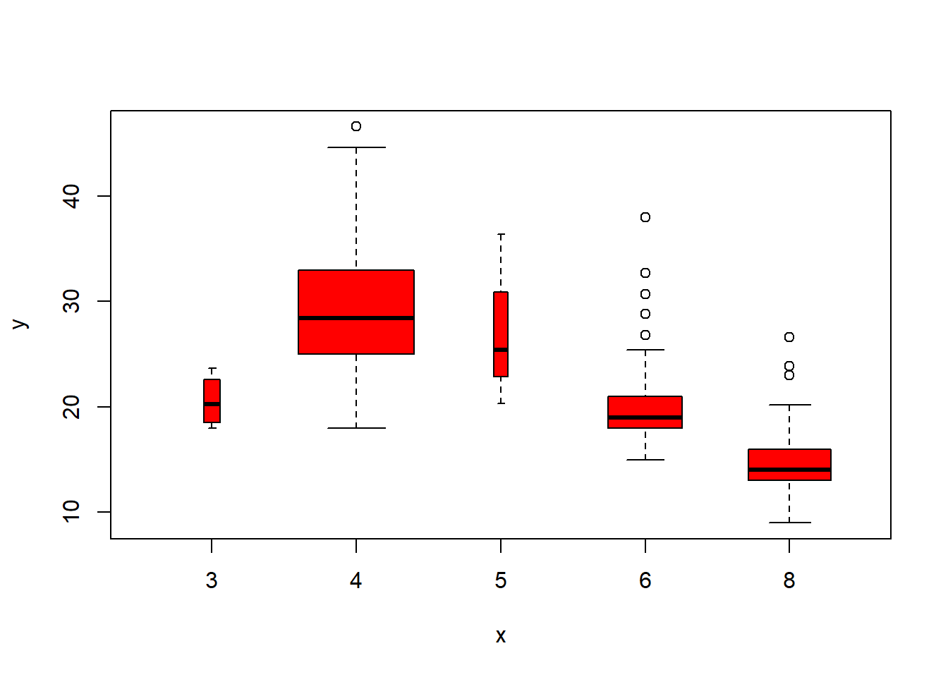

plot(cylinders, mpg, col="red", varwidth=T,horizontal=T)

plot(cylinders, mpg, col="red", varwidth=T, xlab="cylinders", ylab="MPG")

hist(mpg)

hist(mpg,col=2)

hist(mpg,col=2,breaks=15)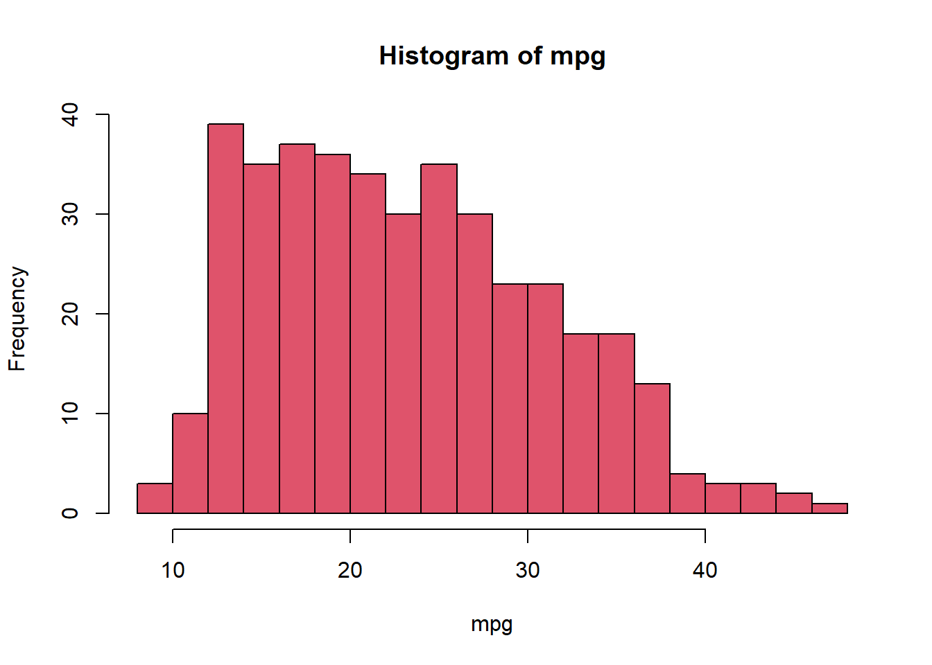

#pairs(Auto)
pairs(~ mpg + displacement + horsepower + weight + acceleration, Auto)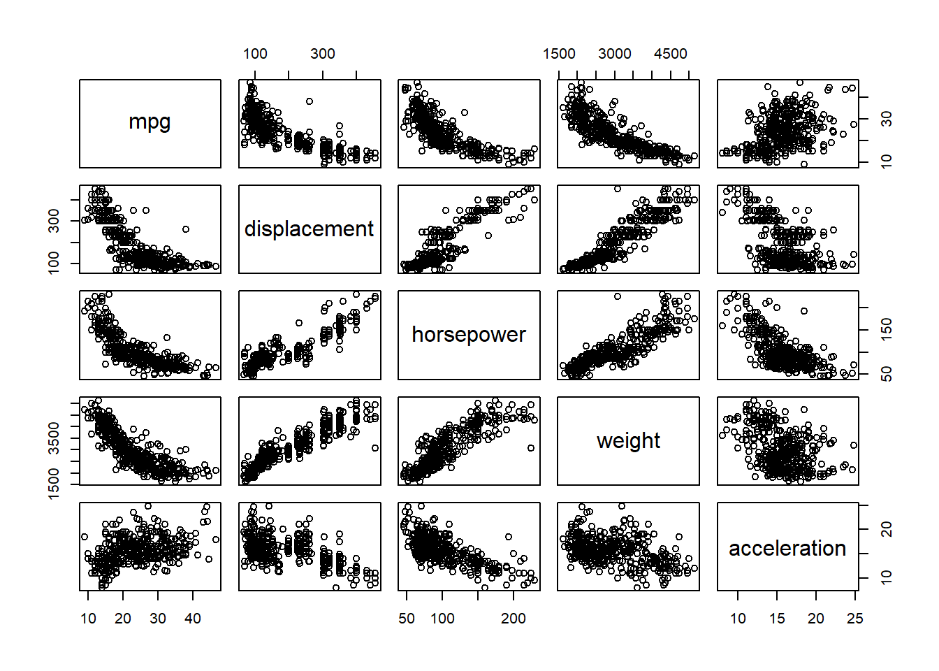

plot(horsepower,mpg)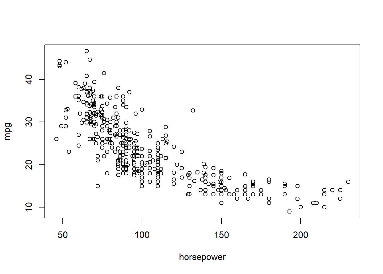

# identify(horsepower,mpg,name) # Interactive: point and click the dot to identify cases
summary(Auto)

      mpg          cylinders      displacement     horsepower        weight    
 Min.   : 9.00   Min.   :3.000   Min.   : 68.0   Min.   : 46.0   Min.   :1613  
 1st Qu.:17.50   1st Qu.:4.000   1st Qu.:104.0   1st Qu.: 75.0   1st Qu.:2223  
 Median :23.00   Median :4.000   Median :146.0   Median : 93.5   Median :2800  
 Mean   :23.52   Mean   :5.458   Mean   :193.5   Mean   :104.5   Mean   :2970  
 3rd Qu.:29.00   3rd Qu.:8.000   3rd Qu.:262.0   3rd Qu.:126.0   3rd Qu.:3609  
 Max.   :46.60   Max.   :8.000   Max.   :455.0   Max.   :230.0   Max.   :5140  
                                                 NA's   :5                     
  acceleration        year           origin          name          
 Min.   : 8.00   Min.   :70.00   Min.   :1.000   Length:397        
 1st Qu.:13.80   1st Qu.:73.00   1st Qu.:1.000   Class :character  
 Median :15.50   Median :76.00   Median :1.000   Mode  :character  
 Mean   :15.56   Mean   :75.99   Mean   :1.574                     
 3rd Qu.:17.10   3rd Qu.:79.00   3rd Qu.:2.000                     
 Max.   :24.80   Max.   :82.00   Max.   :3.000

summary(mpg)

   Min. 1st Qu.  Median    Mean 3rd Qu.    Max. 
   9.00   17.50   23.00   23.52   29.00   46.60

Linear Regression

ptbu=c("MASS","ISLR")
install.packages(ptbu, repos='http://cran.us.r-project.org')

Installing packages into 'C:/Users/akbar/AppData/Local/R/win-library/4.5'
(as 'lib' is unspecified)

package 'MASS' successfully unpacked and MD5 sums checked
package 'ISLR' successfully unpacked and MD5 sums checked

The downloaded binary packages are in
    C:\Users\akbar\AppData\Local\Temp\Rtmp4iJomc\downloaded_packages

lapply(ptbu, require, character.only = TRUE)

Loading required package: MASS

Warning: package 'MASS' was built under R version 4.5.3

Loading required package: ISLR

Warning: package 'ISLR' was built under R version 4.5.3


Attaching package: 'ISLR'

The following object is masked _by_ '.GlobalEnv':

    Auto

[[1]]
[1] TRUE

[[2]]
[1] TRUE

library(MASS)
library(ISLR)

# Simple Linear Regression

# fix(Boston)
names(Boston)

 [1] "crim"    "zn"      "indus"   "chas"    "nox"     "rm"      "age"    
 [8] "dis"     "rad"     "tax"     "ptratio" "black"   "lstat"   "medv"

# lm.fit=lm(medv~lstat)
attach(Boston)
lm.fit=lm(medv~lstat,data=Boston)
attach(Boston)

The following objects are masked from Boston (pos = 3):

    age, black, chas, crim, dis, indus, lstat, medv, nox, ptratio, rad,
    rm, tax, zn

lm.fit=lm(medv~lstat)
lm.fit


Call:
lm(formula = medv ~ lstat)

Coefficients:
(Intercept)        lstat  
      34.55        -0.95

summary(lm.fit)


Call:
lm(formula = medv ~ lstat)

Residuals:
    Min      1Q  Median      3Q     Max 
-15.168  -3.990  -1.318   2.034  24.500 

Coefficients:
            Estimate Std. Error t value Pr(>|t|)    
(Intercept) 34.55384    0.56263   61.41   <2e-16 ***
lstat       -0.95005    0.03873  -24.53   <2e-16 ***
---
Signif. codes:  0 '***' 0.001 '**' 0.01 '*' 0.05 '.' 0.1 ' ' 1

Residual standard error: 6.216 on 504 degrees of freedom
Multiple R-squared:  0.5441,    Adjusted R-squared:  0.5432 
F-statistic: 601.6 on 1 and 504 DF,  p-value: < 2.2e-16

names(lm.fit)

 [1] "coefficients"  "residuals"     "effects"       "rank"         
 [5] "fitted.values" "assign"        "qr"            "df.residual"  
 [9] "xlevels"       "call"          "terms"         "model"

coef(lm.fit)

(Intercept)       lstat 
 34.5538409  -0.9500494

confint(lm.fit)

                2.5 %     97.5 %
(Intercept) 33.448457 35.6592247
lstat       -1.026148 -0.8739505

predict(lm.fit,data.frame(lstat=(c(5,10,15))), interval="confidence")

       fit      lwr      upr
1 29.80359 29.00741 30.59978
2 25.05335 24.47413 25.63256
3 20.30310 19.73159 20.87461

predict(lm.fit,data.frame(lstat=(c(5,10,15))), interval="prediction")

       fit       lwr      upr
1 29.80359 17.565675 42.04151
2 25.05335 12.827626 37.27907
3 20.30310  8.077742 32.52846

# What is the differnce between "conference" and "prediction" difference?

plot(lstat,medv)
abline(lm.fit)
abline(lm.fit,lwd=3)
abline(lm.fit,lwd=3,col="red")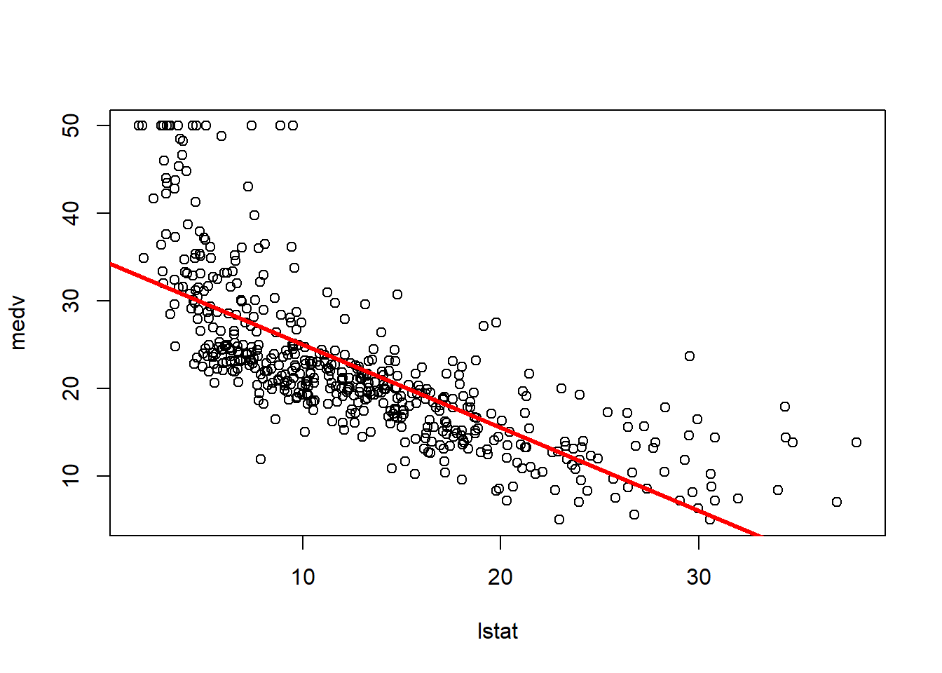

plot(lstat,medv,col="red")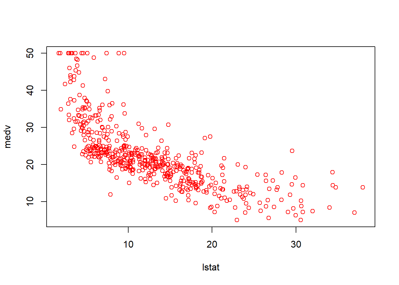

plot(lstat,medv,pch=16)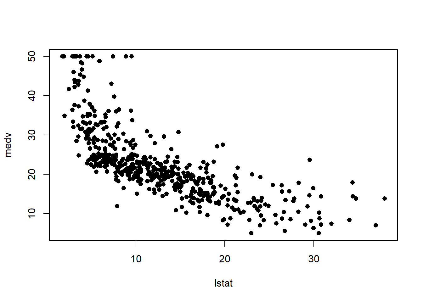

plot(lstat,medv,pch="+")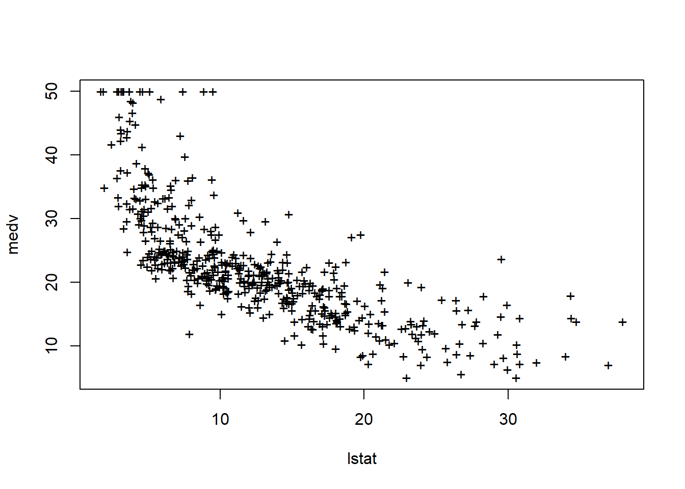

plot(1:20,1:20,pch=1:20)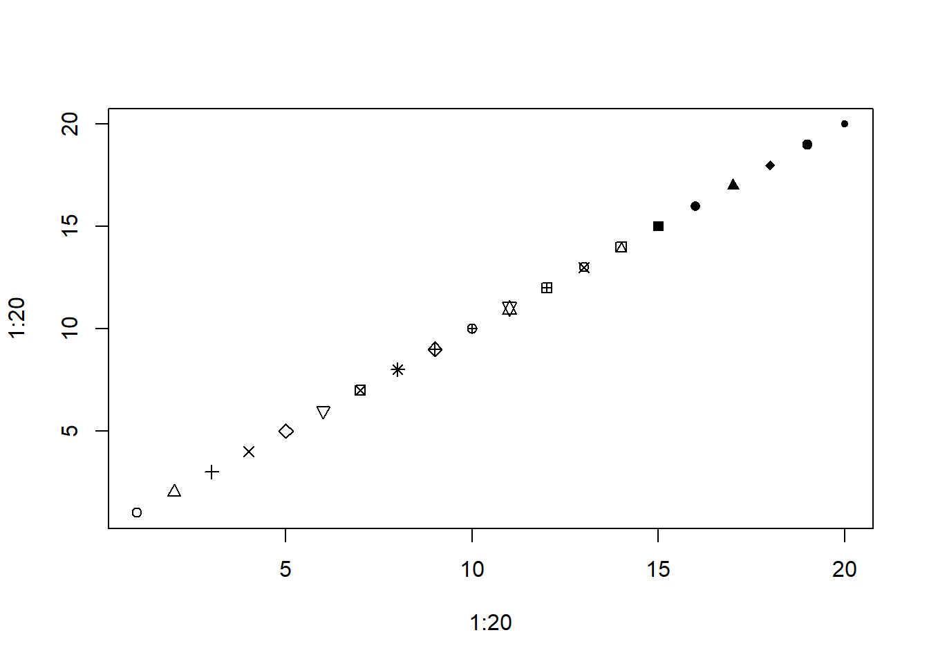

par(mfrow=c(2,2))
plot(lm.fit)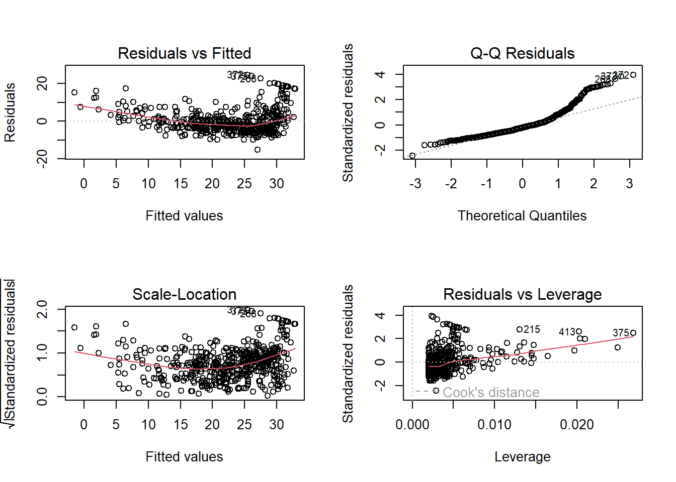

plot(predict(lm.fit), residuals(lm.fit))
plot(predict(lm.fit), rstudent(lm.fit))
plot(hatvalues(lm.fit))
which.max(hatvalues(lm.fit))

375 
375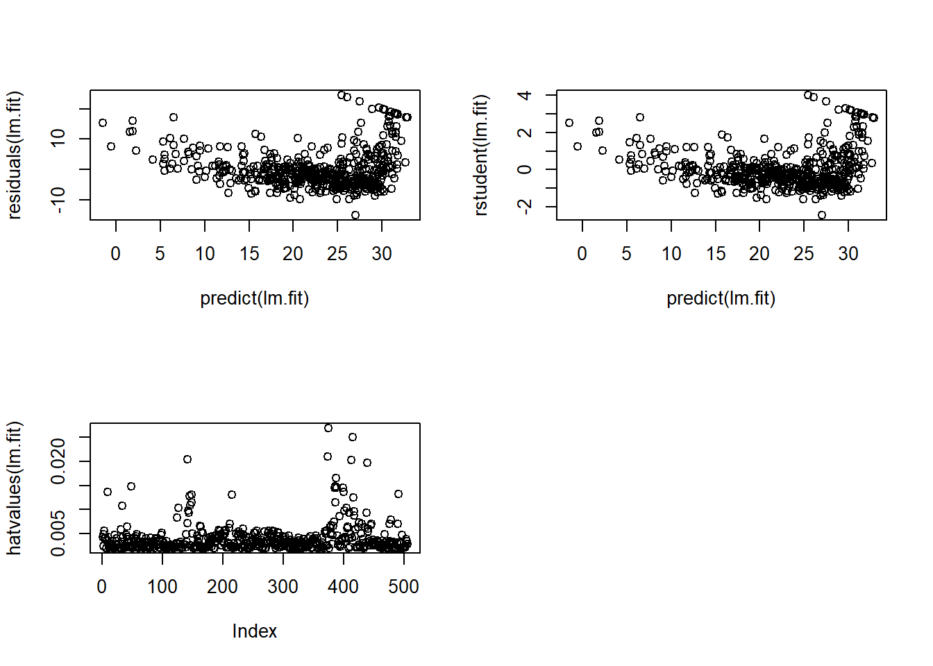

Multiple Linear Regression

lm.fit=lm(medv~lstat+age,data=Boston)
summary(lm.fit)


Call:
lm(formula = medv ~ lstat + age, data = Boston)

Residuals:
    Min      1Q  Median      3Q     Max 
-15.981  -3.978  -1.283   1.968  23.158 

Coefficients:
            Estimate Std. Error t value Pr(>|t|)    
(Intercept) 33.22276    0.73085  45.458  < 2e-16 ***
lstat       -1.03207    0.04819 -21.416  < 2e-16 ***
age          0.03454    0.01223   2.826  0.00491 ** 
---
Signif. codes:  0 '***' 0.001 '**' 0.01 '*' 0.05 '.' 0.1 ' ' 1

Residual standard error: 6.173 on 503 degrees of freedom
Multiple R-squared:  0.5513,    Adjusted R-squared:  0.5495 
F-statistic:   309 on 2 and 503 DF,  p-value: < 2.2e-16

lm.fit=lm(medv~.,data=Boston)
summary(lm.fit)


Call:
lm(formula = medv ~ ., data = Boston)

Residuals:
    Min      1Q  Median      3Q     Max 
-15.595  -2.730  -0.518   1.777  26.199 

Coefficients:
              Estimate Std. Error t value Pr(>|t|)    
(Intercept)  3.646e+01  5.103e+00   7.144 3.28e-12 ***
crim        -1.080e-01  3.286e-02  -3.287 0.001087 ** 
zn           4.642e-02  1.373e-02   3.382 0.000778 ***
indus        2.056e-02  6.150e-02   0.334 0.738288    
chas         2.687e+00  8.616e-01   3.118 0.001925 ** 
nox         -1.777e+01  3.820e+00  -4.651 4.25e-06 ***
rm           3.810e+00  4.179e-01   9.116  < 2e-16 ***
age          6.922e-04  1.321e-02   0.052 0.958229    
dis         -1.476e+00  1.995e-01  -7.398 6.01e-13 ***
rad          3.060e-01  6.635e-02   4.613 5.07e-06 ***
tax         -1.233e-02  3.760e-03  -3.280 0.001112 ** 
ptratio     -9.527e-01  1.308e-01  -7.283 1.31e-12 ***
black        9.312e-03  2.686e-03   3.467 0.000573 ***
lstat       -5.248e-01  5.072e-02 -10.347  < 2e-16 ***
---
Signif. codes:  0 '***' 0.001 '**' 0.01 '*' 0.05 '.' 0.1 ' ' 1

Residual standard error: 4.745 on 492 degrees of freedom
Multiple R-squared:  0.7406,    Adjusted R-squared:  0.7338 
F-statistic: 108.1 on 13 and 492 DF,  p-value: < 2.2e-16

library(car)

Loading required package: carData

Warning: package 'carData' was built under R version 4.5.2

vif(lm.fit)

    crim       zn    indus     chas      nox       rm      age      dis 
1.792192 2.298758 3.991596 1.073995 4.393720 1.933744 3.100826 3.955945 
     rad      tax  ptratio    black    lstat 
7.484496 9.008554 1.799084 1.348521 2.941491

lm.fit1=lm(medv~.-age,data=Boston)
summary(lm.fit1)


Call:
lm(formula = medv ~ . - age, data = Boston)

Residuals:
     Min       1Q   Median       3Q      Max 
-15.6054  -2.7313  -0.5188   1.7601  26.2243 

Coefficients:
              Estimate Std. Error t value Pr(>|t|)    
(Intercept)  36.436927   5.080119   7.172 2.72e-12 ***
crim         -0.108006   0.032832  -3.290 0.001075 ** 
zn            0.046334   0.013613   3.404 0.000719 ***
indus         0.020562   0.061433   0.335 0.737989    
chas          2.689026   0.859598   3.128 0.001863 ** 
nox         -17.713540   3.679308  -4.814 1.97e-06 ***
rm            3.814394   0.408480   9.338  < 2e-16 ***
dis          -1.478612   0.190611  -7.757 5.03e-14 ***
rad           0.305786   0.066089   4.627 4.75e-06 ***
tax          -0.012329   0.003755  -3.283 0.001099 ** 
ptratio      -0.952211   0.130294  -7.308 1.10e-12 ***
black         0.009321   0.002678   3.481 0.000544 ***
lstat        -0.523852   0.047625 -10.999  < 2e-16 ***
---
Signif. codes:  0 '***' 0.001 '**' 0.01 '*' 0.05 '.' 0.1 ' ' 1

Residual standard error: 4.74 on 493 degrees of freedom
Multiple R-squared:  0.7406,    Adjusted R-squared:  0.7343 
F-statistic: 117.3 on 12 and 493 DF,  p-value: < 2.2e-16

lm.fit1=update(lm.fit, ~.-age)

Non-linear Transformations of the Predictors

lm.fit2=lm(medv~lstat+I(lstat^2))
summary(lm.fit2)


Call:
lm(formula = medv ~ lstat + I(lstat^2))

Residuals:
     Min       1Q   Median       3Q      Max 
-15.2834  -3.8313  -0.5295   2.3095  25.4148 

Coefficients:
             Estimate Std. Error t value Pr(>|t|)    
(Intercept) 42.862007   0.872084   49.15   <2e-16 ***
lstat       -2.332821   0.123803  -18.84   <2e-16 ***
I(lstat^2)   0.043547   0.003745   11.63   <2e-16 ***
---
Signif. codes:  0 '***' 0.001 '**' 0.01 '*' 0.05 '.' 0.1 ' ' 1

Residual standard error: 5.524 on 503 degrees of freedom
Multiple R-squared:  0.6407,    Adjusted R-squared:  0.6393 
F-statistic: 448.5 on 2 and 503 DF,  p-value: < 2.2e-16

lm.fit=lm(medv~lstat)
anova(lm.fit,lm.fit2)

Analysis of Variance Table

Model 1: medv ~ lstat
Model 2: medv ~ lstat + I(lstat^2)
  Res.Df   RSS Df Sum of Sq     F    Pr(>F)    
1    504 19472                                 
2    503 15347  1    4125.1 135.2 < 2.2e-16 ***
---
Signif. codes:  0 '***' 0.001 '**' 0.01 '*' 0.05 '.' 0.1 ' ' 1

par(mfrow=c(2,2))
plot(lm.fit2)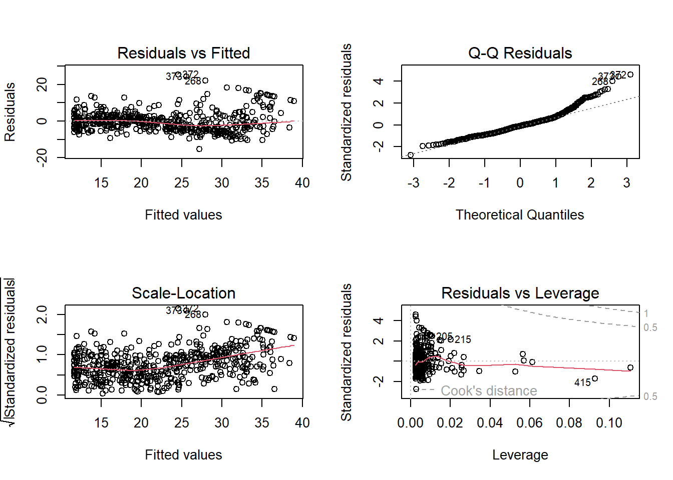

lm.fit5=lm(medv~poly(lstat,5))
summary(lm.fit5)


Call:
lm(formula = medv ~ poly(lstat, 5))

Residuals:
     Min       1Q   Median       3Q      Max 
-13.5433  -3.1039  -0.7052   2.0844  27.1153 

Coefficients:
                 Estimate Std. Error t value Pr(>|t|)    
(Intercept)       22.5328     0.2318  97.197  < 2e-16 ***
poly(lstat, 5)1 -152.4595     5.2148 -29.236  < 2e-16 ***
poly(lstat, 5)2   64.2272     5.2148  12.316  < 2e-16 ***
poly(lstat, 5)3  -27.0511     5.2148  -5.187 3.10e-07 ***
poly(lstat, 5)4   25.4517     5.2148   4.881 1.42e-06 ***
poly(lstat, 5)5  -19.2524     5.2148  -3.692 0.000247 ***
---
Signif. codes:  0 '***' 0.001 '**' 0.01 '*' 0.05 '.' 0.1 ' ' 1

Residual standard error: 5.215 on 500 degrees of freedom
Multiple R-squared:  0.6817,    Adjusted R-squared:  0.6785 
F-statistic: 214.2 on 5 and 500 DF,  p-value: < 2.2e-16

summary(lm(medv~log(rm),data=Boston))


Call:
lm(formula = medv ~ log(rm), data = Boston)

Residuals:
    Min      1Q  Median      3Q     Max 
-19.487  -2.875  -0.104   2.837  39.816 

Coefficients:
            Estimate Std. Error t value Pr(>|t|)    
(Intercept)  -76.488      5.028  -15.21   <2e-16 ***
log(rm)       54.055      2.739   19.73   <2e-16 ***
---
Signif. codes:  0 '***' 0.001 '**' 0.01 '*' 0.05 '.' 0.1 ' ' 1

Residual standard error: 6.915 on 504 degrees of freedom
Multiple R-squared:  0.4358,    Adjusted R-squared:  0.4347 
F-statistic: 389.3 on 1 and 504 DF,  p-value: < 2.2e-16

Qualitative Predictors

# fix(Carseats)
names(Carseats)

 [1] "Sales"       "CompPrice"   "Income"      "Advertising" "Population" 
 [6] "Price"       "ShelveLoc"   "Age"         "Education"   "Urban"      
[11] "US"

lm.fit=lm(Sales~.+Income:Advertising+Price:Age,data=Carseats)
summary(lm.fit)


Call:
lm(formula = Sales ~ . + Income:Advertising + Price:Age, data = Carseats)

Residuals:
    Min      1Q  Median      3Q     Max 
-2.9208 -0.7503  0.0177  0.6754  3.3413 

Coefficients:
                     Estimate Std. Error t value Pr(>|t|)    
(Intercept)         6.5755654  1.0087470   6.519 2.22e-10 ***
CompPrice           0.0929371  0.0041183  22.567  < 2e-16 ***
Income              0.0108940  0.0026044   4.183 3.57e-05 ***
Advertising         0.0702462  0.0226091   3.107 0.002030 ** 
Population          0.0001592  0.0003679   0.433 0.665330    
Price              -0.1008064  0.0074399 -13.549  < 2e-16 ***
ShelveLocGood       4.8486762  0.1528378  31.724  < 2e-16 ***
ShelveLocMedium     1.9532620  0.1257682  15.531  < 2e-16 ***
Age                -0.0579466  0.0159506  -3.633 0.000318 ***
Education          -0.0208525  0.0196131  -1.063 0.288361    
UrbanYes            0.1401597  0.1124019   1.247 0.213171    
USYes              -0.1575571  0.1489234  -1.058 0.290729    
Income:Advertising  0.0007510  0.0002784   2.698 0.007290 ** 
Price:Age           0.0001068  0.0001333   0.801 0.423812    
---
Signif. codes:  0 '***' 0.001 '**' 0.01 '*' 0.05 '.' 0.1 ' ' 1

Residual standard error: 1.011 on 386 degrees of freedom
Multiple R-squared:  0.8761,    Adjusted R-squared:  0.8719 
F-statistic:   210 on 13 and 386 DF,  p-value: < 2.2e-16

attach(Carseats)
contrasts(ShelveLoc)

       Good Medium
Bad       0      0
Good      1      0
Medium    0      1

Interaction Terms (including interaction and single effects)

summary(lm(medv~lstat*age,data=Boston))


Call:
lm(formula = medv ~ lstat * age, data = Boston)

Residuals:
    Min      1Q  Median      3Q     Max 
-15.806  -4.045  -1.333   2.085  27.552 

Coefficients:
              Estimate Std. Error t value Pr(>|t|)    
(Intercept) 36.0885359  1.4698355  24.553  < 2e-16 ***
lstat       -1.3921168  0.1674555  -8.313 8.78e-16 ***
age         -0.0007209  0.0198792  -0.036   0.9711    
lstat:age    0.0041560  0.0018518   2.244   0.0252 *  
---
Signif. codes:  0 '***' 0.001 '**' 0.01 '*' 0.05 '.' 0.1 ' ' 1

Residual standard error: 6.149 on 502 degrees of freedom
Multiple R-squared:  0.5557,    Adjusted R-squared:  0.5531 
F-statistic: 209.3 on 3 and 502 DF,  p-value: < 2.2e-16

R4DS Section 3.5 Illustration

# Import the TEDS 2016 data in Stata format using the haven package
##install.packages("haven")

library(haven)

Warning: package 'haven' was built under R version 4.5.2

TEDS_2016 <- read_stata("https://github.com/datageneration/home/blob/master/DataProgramming/data/TEDS_2016.dta?raw=true")

# Prepare the analyze the Party ID variable 
# Assign label to the values (1=KMT, 2=DPP, 3=NP, 4=PFP, 5=TSU, 6=NPP, 7="NA")

TEDS_2016$PartyID <- factor(TEDS_2016$PartyID, labels=c("KMT","DPP","NP","PFP", "TSU", "NPP","NA"))

# Check the variable
attach(TEDS_2016)

The following object is masked from Carseats:

    Age

The following object is masked from Boston (pos = 7):

    age

The following object is masked from Boston (pos = 8):

    age

head(PartyID)

[1] NA  NA  KMT NA  NA  DPP
Levels: KMT DPP NP PFP TSU NPP NA

tail(PartyID)

[1] NA  NA  DPP NA  NA  NA 
Levels: KMT DPP NP PFP TSU NPP NA

# Run a frequency table of the Party ID variable using the descr package
##install.packages("descr")
library(descr)

Warning: package 'descr' was built under R version 4.5.2

freq(TEDS_2016$PartyID)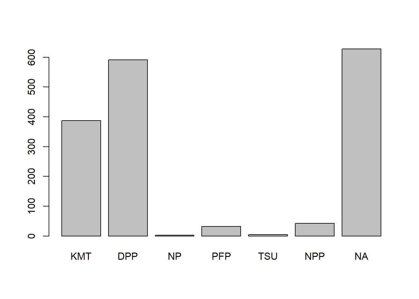

TEDS_2016$PartyID 
      Frequency  Percent
KMT         388  22.9586
DPP         591  34.9704
NP            3   0.1775
PFP          32   1.8935
TSU           5   0.2959
NPP          43   2.5444
NA          628  37.1598
Total      1690 100.0000

# Plot the Party ID variable
library(ggplot2)

Warning: package 'ggplot2' was built under R version 4.5.3


Attaching package: 'ggplot2'

The following object is masked from 'Auto':

    mpg

ggplot(TEDS_2016, aes(PartyID)) + 
  geom_bar()

ggplot(TEDS_2016, aes(PartyID)) + 
  geom_bar(aes(y = (..count..)/sum(..count..))) + 
  scale_y_continuous(labels=scales::percent) +
  ylab("Party Support (%)") + 
  xlab("Taiwan Political Parties")

Warning: The dot-dot notation (`..count..`) was deprecated in ggplot2 3.4.0.
ℹ Please use `after_stat(count)` instead.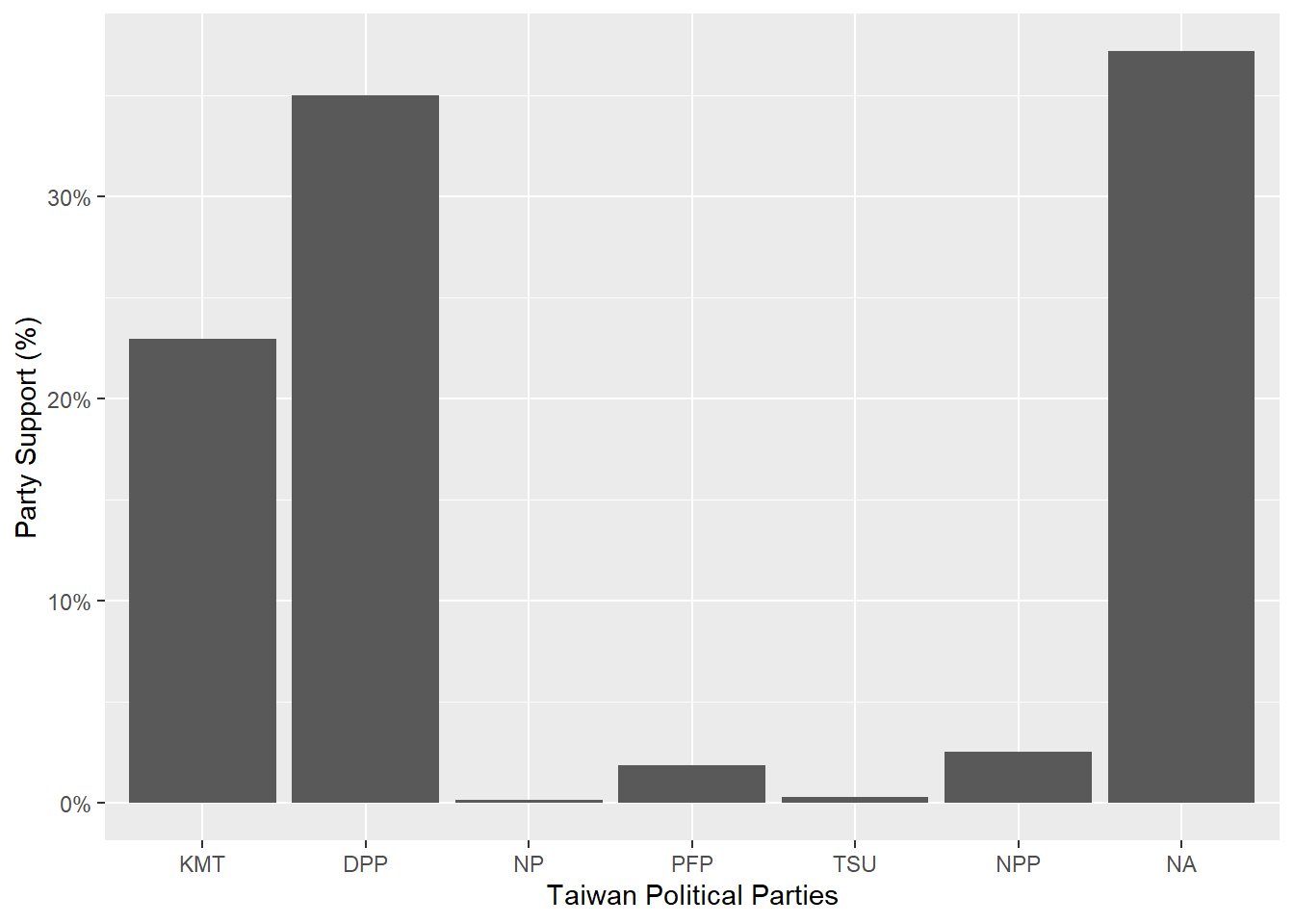

ggplot(TEDS_2016, aes(PartyID)) + 
  geom_bar(aes(y = (..count..)/sum(..count..),fill=PartyID)) + 
  scale_y_continuous(labels=scales::percent) +
  ylab("Party Support (%)") + 
  xlab("Taiwan Political Parties") +
  theme_bw()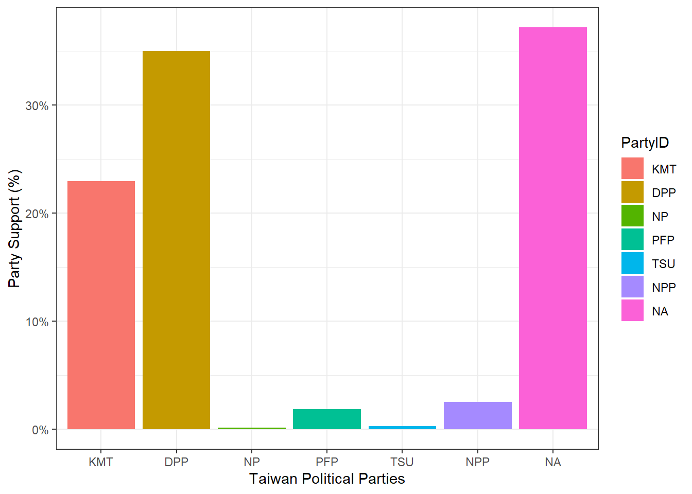

ggplot(TEDS_2016, aes(PartyID)) + 
  geom_bar(aes(y = (..count..)/sum(..count..),fill=PartyID)) + 
  scale_y_continuous(labels=scales::percent) +
  ylab("Party Support (%)") + 
  xlab("Taiwan Political Parties") +
  theme_bw() +
  scale_fill_manual(values=c("steel blue","forestgreen","khaki1","orange","goldenrod","yellow","grey"))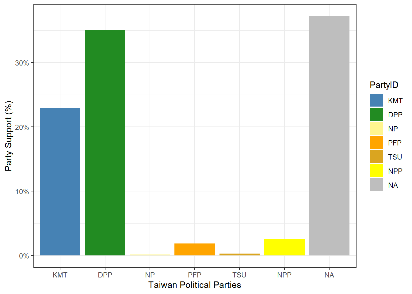

##install.packages("tidyverse")
library(tidyverse)

Warning: package 'tidyverse' was built under R version 4.5.3

Warning: package 'tidyr' was built under R version 4.5.3

Warning: package 'readr' was built under R version 4.5.3

Warning: package 'dplyr' was built under R version 4.5.3

Warning: package 'lubridate' was built under R version 4.5.2

── Attaching core tidyverse packages ──────────────────────── tidyverse 2.0.0 ──
✔ dplyr     1.2.1     ✔ readr     2.2.0
✔ forcats   1.0.0     ✔ stringr   1.5.1
✔ lubridate 1.9.4     ✔ tibble    3.3.0
✔ purrr     1.1.0     ✔ tidyr     1.3.2
── Conflicts ────────────────────────────────────────── tidyverse_conflicts() ──
✖ dplyr::filter() masks stats::filter()
✖ dplyr::lag()    masks stats::lag()
✖ dplyr::recode() masks car::recode()
✖ dplyr::select() masks MASS::select()
✖ purrr::some()   masks car::some()
ℹ Use the conflicted package (<http://conflicted.r-lib.org/>) to force all conflicts to become errors

TEDS_2016 %>% 
  count(PartyID) %>% 
  mutate(perc = n / nrow(TEDS_2016)) -> T2
ggplot(T2, aes(x = reorder(PartyID, -perc),y = perc,fill=PartyID)) + 
  geom_bar(stat = "identity") +
  ylab("Party Support (%)") + 
  xlab("Taiwan Political Parties") +
  theme_bw() +
  scale_fill_manual(values=c("steel blue","forestgreen","khaki1","orange","goldenrod","yellow","grey"))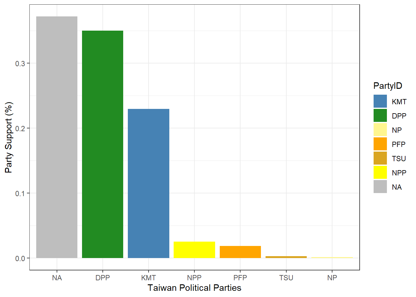

The TEDS2016 dataset is a list of information that contains data on Taiwanese political parties and its support. Parties such as the Democratic Progressive Party (DPP), Kuomintang (KMT), New Power Party (NPP), People’s First Party (PFP), Taiwan Solidarity Party (TSU), and New Party (NP), have received public support. While the DPP and KMT have the most support, most of the data however is missing, which are labeled as N/A.

In order to deal with missing data, the N/A category may be left as its own category, demonstrating that there is a number of non-responses. Another way to deal with missing data is to exclude the N/A category to remove any bias.

In the TEDS_2016 dataset, I explore the relationship between Tondu and other variables such as female, DPP, age, income, edu, Taiwanese and Econ_worse. Tondu is a variable that represents a position focused on unification and independence. Since the dataset already provides the variables, I’m going to use AI models such as ChatGBT to assist me with the first code for a close up comparison between Tondu and female. Following after, I will continue the coding with Tondu and the rest.

table(TEDS_2016$Tondu, TEDS_2016$female)

table(TEDS_2016$Tondu, TEDS_2016$DPP)

table(TEDS_2016$Tondu, TEDS_2016$age)

   
    20 21 22 23 24 25 26 27 28 29 30 31 32 33 34 35 36 37 38 39 40 41 42 43 44
  1  0  0  0  0  1  0  0  0  0  1  0  0  1  1  0  0  0  0  1  0  0  1  0  0  0
  2  0  0  0  1  2  1  0  2  1  1  0  0  0  0  4  5  4  4  2  3  3  3  3  1  3
  3  0  9 11  9 11 12 12  5 10 11  9 10  6  7 13 13  6 19 13  9 14  9 16 10  8
  4  0  6  5  3  2  4  4  3  3  4  4  2  3  2 11  5  3  3  3  6  6  2  6  4  6
  5  2 14 18 11 13 10 11 14  8  7 11  8  8  3 13  9  8  5  8  7  6  9  6  5 10
  6  0  6  3  2  4  1  1  0  2  1  1  2  2  0  3  4  2  4  3  1  2  2  2  2  2
  9  0  0  0  0  0  0  1  0  1  0  0  1  0  2  2  0  1  0  1  1  0  1  1  2  1
   
    45 46 47 48 49 50 51 52 53 54 55 56 57 58 59 60 61 62 63 64 65 66 67 68 69
  1  0  0  0  1  0  0  0  0  0  0  1  2  1  0  3  1  1  0  0  0  0  1  1  1  1
  2  5  3  6  4  2  3  1  9  6  2  6  3  5  2  4 11  4  2  3  1  6  4  4  7  4
  3  8 17 13 16 22 15 13 12  8  8 10 17 13  9 12 10  8 11  6 10  3 10  8  6  5
  4  3  8  7  8  8  5 11  3  8  7  6  6 12  9  5  5 12  6  6 12 12  6  5  4  8
  5  4  6  7  6  5  7  4  6  3  6  9  6  6  6 11  9  3  4  3  4  8  2  4  3  1
  6  4  1  1  1  1  1  1  1  1  2  1  3  3  0  1  4  3  1  4  0  1  2  2  0  2
  9  0  0  1  0  3  2  3  1  2  2  7  0  1  2  2  4  2  0  3  6  4  5  4  3  0
   
    70 71 72 73 74 75 76 77 78 79 80 81 82 83 84 85 86 87 88 89 90 91 92 94 95
  1  0  0  1  3  1  0  1  0  0  0  0  0  0  0  0  0  1  0  0  0  0  0  0  0  0
  2  4  1  1  2  1  4  2  1  1  1  1  1  0  0  0  4  1  3  0  1  0  0  0  0  0
  3  3  3  2  1  4  1  1  0  1  1  2  2  1  0  0  0  1  0  0  1  0  0  0  0  0
  4  2  1  7  7  3  4  3  0  1  1  3  0  3  3  2  1  2  0  0  0  0  1  1  1  0
  5  1  2  4  1  3  1  3  1  1  1  1  0  0  0  2  0  1  0  0  0  0  0  0  0  1
  6  0  0  1  1  1  3  2  0  1  0  2  0  1  0  1  1  0  0  0  0  1  0  0  0  0
  9  3  1  3  2  0  3  2  5  4  5  3  3  3  4  0  1  2  1  1  1  1  0  1  0  0
   
    100
  1   0
  2   1
  3   0
  4   0
  5   0
  6   0
  9   0

table(TEDS_2016$Tondu, TEDS_2016$income)

   
     1  2  3  4  5 5.5  6  7  8  9 10
  1  7  3  2  1  0   5  4  0  2  2  1
  2 23 12 11 14 22  20 17 12 16 13 20
  3 47 42 43 34 52  96 48 38 56 36 54
  4 50 25 19 24 18  76 24 20 24 19 29
  5 38 23 23 38 36  52 23 39 35 31 42
  6 27  7  8  7  7  21  7  5  6  4  9
  9 35  7  5  1  5  60  2  1  1  2  2

table(TEDS_2016$Tondu, TEDS_2016$edu)

   
      1   2   3   4   5
  1  10   3  10   1   2
  2  31  14  58  31  45
  3  60  49 157  71 208
  4  71  45  93  36  80
  5  36  30  88  34 192
  6  32  11  31   8  26
  9  82   9  12   5   9

table(TEDS_2016$Tondu, TEDS_2016$Taiwanese)

table(TEDS_2016$Tondu, TEDS_2016$Econ_worse)

First, the relationship between Tondu and the female variable shows a clear association, suggesting that women play an important role in shaping attitudes toward unification and independence in Taiwan. Second, there is a strong relationship between Tondu and the DPP variable, as respondents who strongly identify and support the DPP are more likely to favor independence-oriented positions, while non-DPP supporters tend to be more concentrated in status quo or unification positions. Third, the relationships between Tondu and age, income, and education are more difficult to interpret because these variables are continuous, making simple contingency tables inappropriate and complex. Fourth, the Taiwanese variable is strongly associated with Tondu, indicating that national identity plays a crucial role in preferences regarding unification and independence. Lastly, economic perceptions (Econ_worse) are also associated with Tondu, suggesting that views about economic conditions may influence attitudes toward unification and independence.

table(TEDS_2016$Tondu, TEDS_2016$votetsai)

The votetsai variable focuses on the vote for the DPP candidate Tsai Ing-wen. The data indicates that there is a strong relationship between these two variables. Respondents that voted for Tsai Ing-wen are more likely to favor independence and unification than those that do not support the candidate.

library(haven)
TEDS_2016 <- read_stata("https://github.com/datageneration/home/blob/master/DataProgramming/data/TEDS_2016.dta?raw=true")

TEDS_2016$Tondu<-as.numeric(TEDS_2016$Tondu,labels=c("Unification now”, 
“Status quo, unif. in future”, “Status quo, decide later", "Status quo 
forever", "Status quo, indep. in future", "Independence now”, “No response"))

attach(TEDS_2016)

The following objects are masked from TEDS_2016 (pos = 14):

    age, Age, Arear, Blue, Career, Career8, District, DPP, Econ_worse,
    econworse5, edu, Edu, Ethnic, female, Govt_dont_care,
    Govt_for_public, green, Green, highincome, income, income_nm,
    Independence, Inequality, inequality5, KMT, lowincome,
    Mainland_father, Minnan_father, nI2, No_Party, noparty, north, npp,
    Party, PartyID, pfp, pubwelf5, Sex, South, sq, Taiwanese, Tondu,
    Tondu3, Unification, voteblue, voteblue_nm, votedpp_1, votekmt,
    votekmt_1, votekmt_nm, votetsai, votetsai_all, votetsai_nm,
    whitecollar

The following object is masked from Carseats:

    Age

The following object is masked from Boston (pos = 19):

    age

The following object is masked from Boston (pos = 20):

    age

head(Tondu)

[1] 3 5 3 5 9 4

tail(Tondu)

[1] 2 3 4 4 3 3

library(descr)
freq(TEDS_2016$Tondu)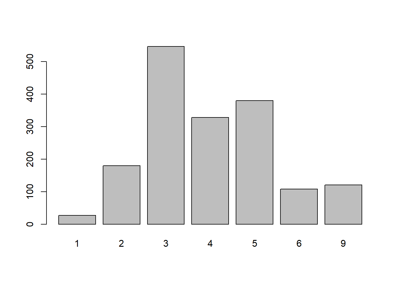

TEDS_2016$Tondu 
      Frequency Percent
1            27   1.598
2           180  10.651
3           546  32.308
4           328  19.408
5           380  22.485
6           108   6.391
9           121   7.160
Total      1690 100.000

library(ggplot2)
ggplot(TEDS_2016, aes(Tondu)) + 
  geom_bar()

ggplot(TEDS_2016, aes(Tondu)) + 
  geom_bar(aes(y = (..count..)/sum(..count..))) + 
  scale_y_continuous(labels=scales::percent) +
  ylab("Share of Respondents (%)") + 
  xlab("Attitudes Toward Unification and Independence (Tondu)")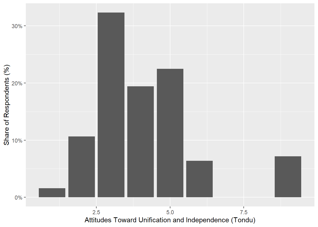

ggplot(TEDS_2016, aes(Tondu)) + 
  geom_bar(aes(y = (..count..)/sum(..count..),fill=Tondu)) + 
  scale_y_continuous(labels=scales::percent) +
  ylab("Share of Respondents (%)") + 
  xlab("Attitudes Toward Unification and Independence (Tondu)") +
  theme_bw()

Warning: The following aesthetics were dropped during statistical transformation: fill.
ℹ This can happen when ggplot fails to infer the correct grouping structure in
  the data.
ℹ Did you forget to specify a `group` aesthetic or to convert a numerical
  variable into a factor?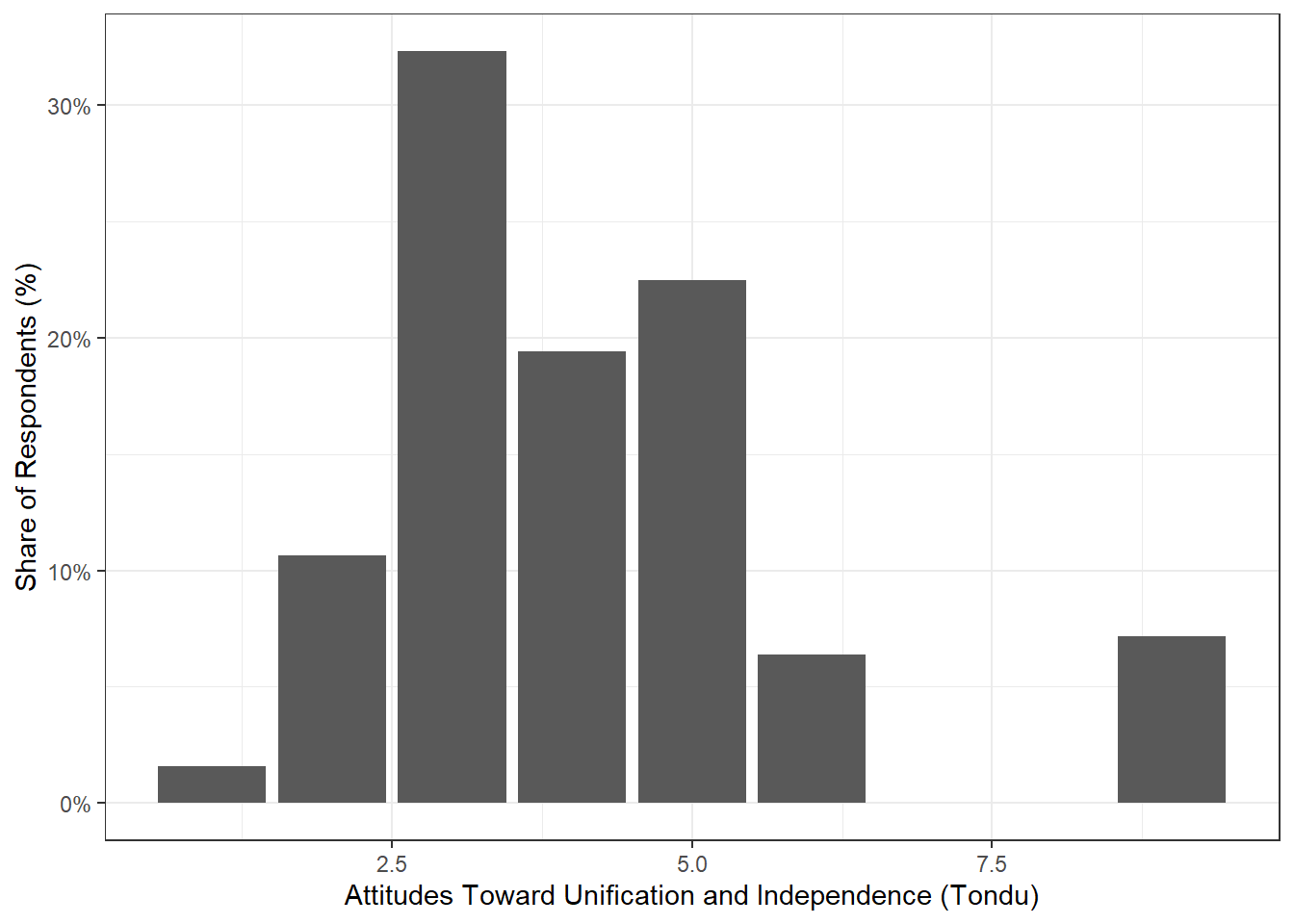

ggplot(TEDS_2016, aes(Tondu)) + 
  geom_bar(aes(y = (..count..)/sum(..count..),fill=Tondu)) + 
  scale_y_continuous(labels=scales::percent) +
  ylab("Share of Respondents (%)") + 
  xlab("Attitudes Toward Unification and Independence (Tondu)") +
  theme_bw() +
  scale_fill_manual(values=c("steel blue","forestgreen","khaki1","orange","goldenrod","yellow","grey"))

Warning: The following aesthetics were dropped during statistical transformation: fill.
ℹ This can happen when ggplot fails to infer the correct grouping structure in
  the data.
ℹ Did you forget to specify a `group` aesthetic or to convert a numerical
  variable into a factor?

library(tidyverse)
library(scales)

Warning: package 'scales' was built under R version 4.5.3


Attaching package: 'scales'

The following object is masked from 'package:purrr':

    discard

The following object is masked from 'package:readr':

    col_factor

# Make Tondu discrete (factor) with labels
TEDS_2016 <- TEDS_2016 %>%
  mutate(
    Tondu = factor(
      Tondu,
      levels = c(1, 2, 3, 4, 5, 6, 7),
      labels = c(
        "Unification now",
        "Status quo, unif. in future",
        "Status quo, decide later",
        "Status quo forever",
        "Status quo, indep. in future",
        "Independence now",
        "No response"
      )
    )
  )

T2 <- TEDS_2016 %>%
  filter(!is.na(Tondu)) %>%
  count(Tondu) %>%
  mutate(perc = n / sum(n))

ggplot(T2, aes(x = reorder(Tondu, -perc), y = perc, fill = Tondu)) + 
  geom_bar(stat = "identity") +
  scale_y_continuous(labels = percent) +
  ylab("Share of Respondents (%)") + 
  xlab("Attitudes Toward Unification and Independence (Tondu)") +
  theme_bw() +
  theme(axis.text.x = element_text(angle = 45, hjust = 1)) +
  scale_fill_manual(values = c(
    "steel blue","forestgreen","khaki1",
    "orange","goldenrod","yellow","grey"
  ))

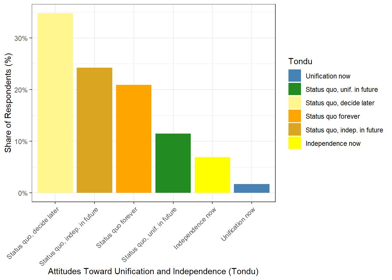
For the final section of the last code (making Tondu discrete (factor) with labels), I used ChatGPT to help troubleshoot and fix errors I was encountering. All other code was reviewed and written by me.