See https://quanteda.io for tutorials and examples.
library(quanteda.textmodels)
Warning: package 'quanteda.textmodels' was built under R version 4.5.3
library(quanteda.textplots)
Warning: package 'quanteda.textplots' was built under R version 4.5.3
library(readr)
Warning: package 'readr' was built under R version 4.5.3
library(ggplot2)
Warning: package 'ggplot2' was built under R version 4.5.3
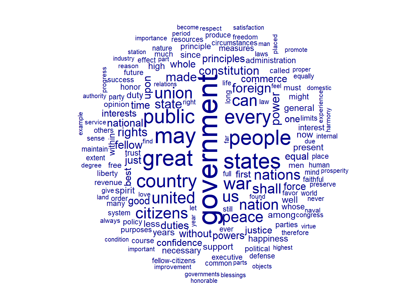
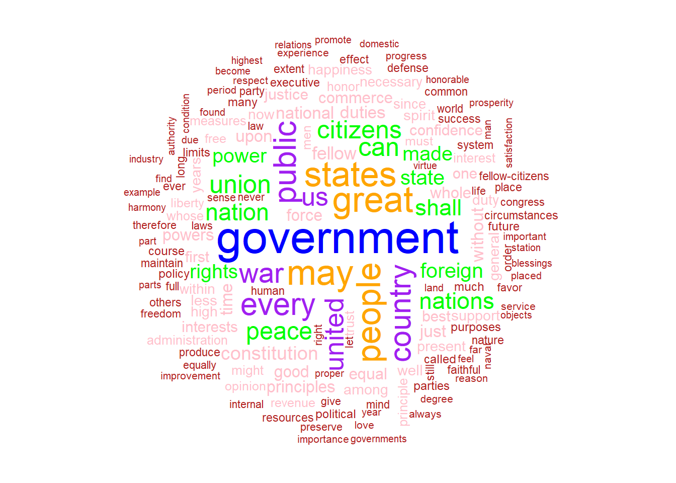
# Wordcloud# based on US presidential inaugural address texts, and metadata (for the corpus), from 1789 to present.dfm_inaug <-corpus_subset(data_corpus_inaugural, Year <=1826) %>%tokens(remove_punct =TRUE) %>%tokens_remove(stopwords('english')) %>%dfm() %>%dfm_trim(min_termfreq =10, verbose =FALSE)set.seed(100)textplot_wordcloud(dfm_inaug)
Document-feature matrix of: 6 documents, 4,625 features (86.44% sparse) and 4 docvars.
features
docs my friends , before i
1953-Eisenhower 0.14582574 0.14582574 4.593511 0.1822822 0.10936930
1957-Eisenhower 0.20975354 0.10487677 6.345045 0.1573152 0.05243838
1961-Kennedy 0.19467878 0.06489293 5.451006 0.1297859 0.32446463
1965-Johnson 0.17543860 0.05847953 5.555556 0.2339181 0.87719298
1969-Nixon 0.28973510 0 5.546358 0.1241722 0.86920530
1973-Nixon 0.05012531 0.05012531 4.812030 0.2005013 0.60150376
features
docs begin the expression of those
1953-Eisenhower 0.03645643 6.234050 0.03645643 5.176814 0.1458257
1957-Eisenhower 0 5.977976 0 5.034085 0.1573152
1961-Kennedy 0.19467878 5.580792 0 4.218040 0.4542505
1965-Johnson 0 4.502924 0 3.333333 0.1754386
1969-Nixon 0 5.629139 0 3.890728 0.4552980
1973-Nixon 0 4.160401 0 3.408521 0.3007519
[ reached max_nfeat ... 4,615 more features ]
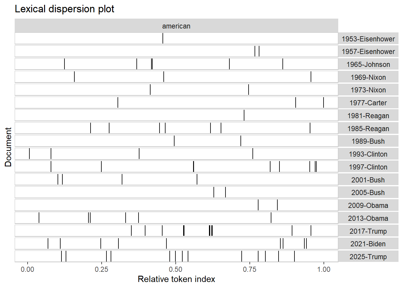
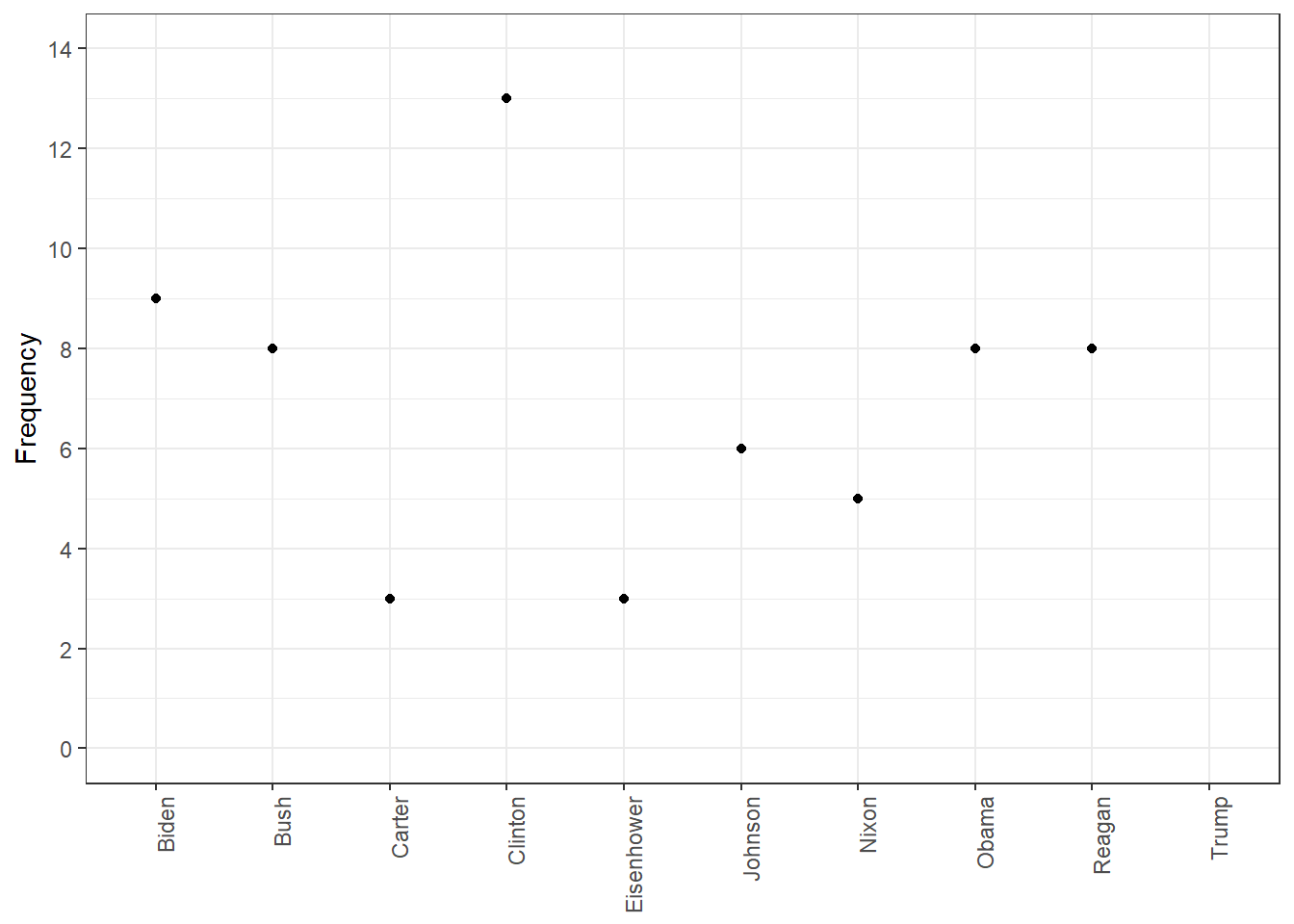
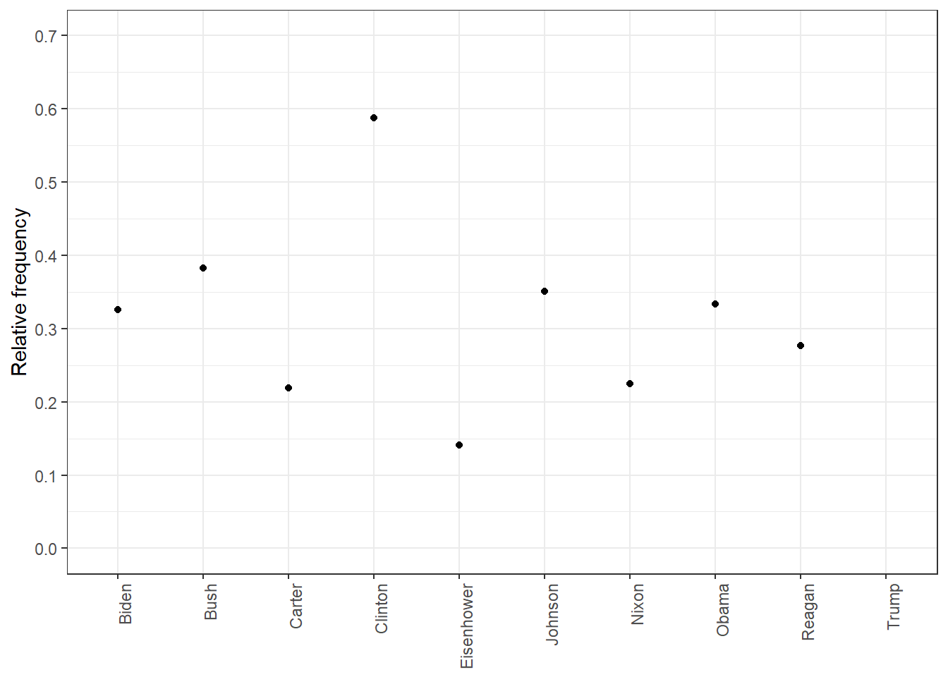
rel_freq <-textstat_frequency(dfm_rel_freq, groups = dfm_rel_freq$President)# Filter the term "american"rel_freq_american <-subset(rel_freq, feature %in%"american") ggplot(rel_freq_american, aes(x = group, y = frequency)) +geom_point() +scale_y_continuous(limits =c(0, 0.7), breaks =c(seq(0, 0.7, 0.1))) +xlab(NULL) +ylab("Relative frequency") +theme(axis.text.x =element_text(angle =90, hjust =1))
Warning: Removed 1 row containing missing values or values outside the scale range
(`geom_point()`).
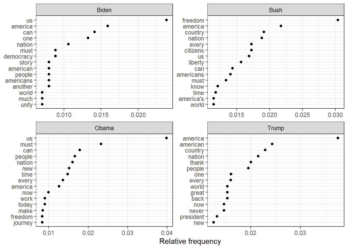
dfm_weight_pres <- data_corpus_inaugural %>%corpus_subset(Year >2000) %>%tokens(remove_punct =TRUE) %>%tokens_remove(stopwords("english")) %>%dfm() %>%dfm_weight(scheme ="prop")# Calculate relative frequency by presidentfreq_weight <-textstat_frequency(dfm_weight_pres, n =15, groups = dfm_weight_pres$President)ggplot(data = freq_weight, aes(x =nrow(freq_weight):1, y = frequency)) +geom_point() +facet_wrap(~ group, scales ="free") +coord_flip() +scale_x_continuous(breaks =nrow(freq_weight):1,labels = freq_weight$feature) +labs(x =NULL, y ="Relative frequency")
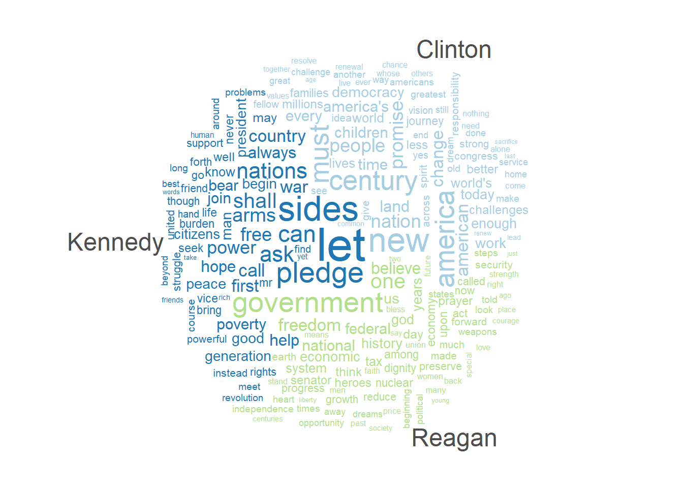
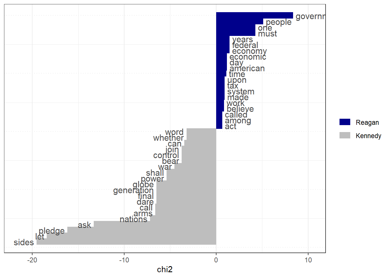
# Only select speeches by Kennedy and Reaganpres_corpus <-corpus_subset(data_corpus_inaugural, President %in%c("Kennedy", "Reagan"))# Create a dfm grouped by presidentpres_dfm <-tokens(pres_corpus, remove_punct =TRUE) %>%tokens_remove(stopwords("english")) %>%tokens_group(groups = President) %>%dfm()# Calculate keyness and determine Reagan as target groupresult_keyness <-textstat_keyness(pres_dfm, target ="Reagan")# Plot estimated word keynesstextplot_keyness(result_keyness)
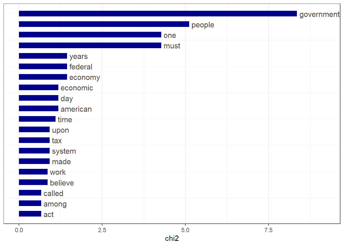
# Plot without the reference text (in this case Obama)textplot_keyness(result_keyness, show_reference =FALSE)
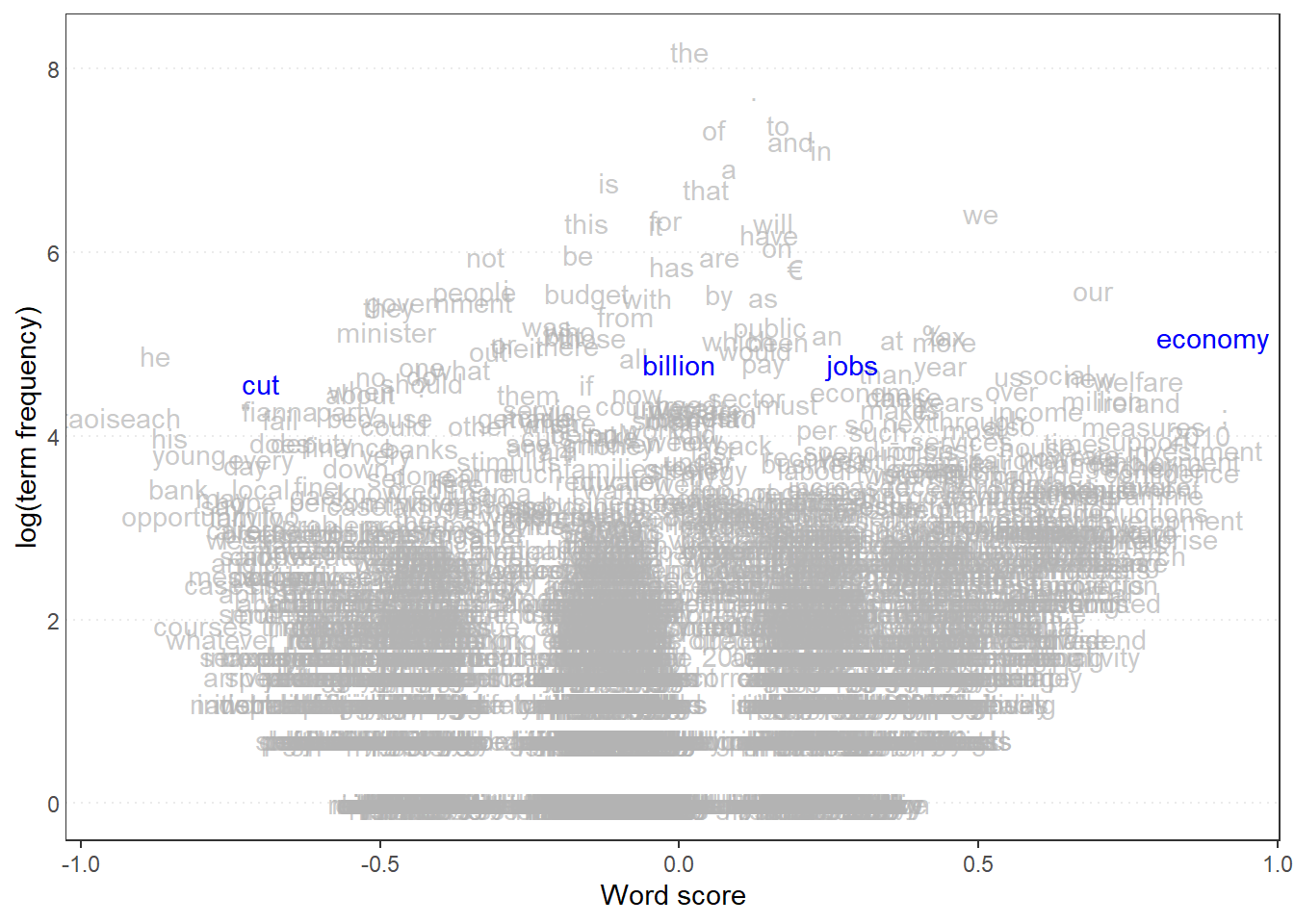
library(quanteda.textmodels)# Irish budget speeches from 2010 (data from quanteda.textmodels)# Transform corpus to dfmdata(data_corpus_irishbudget2010, package ="quanteda.textmodels")ie_dfm <-dfm(tokens(data_corpus_irishbudget2010))# Set reference scoresrefscores <-c(rep(NA, 4), 1, -1, rep(NA, 8))# Predict Wordscores modelws <-textmodel_wordscores(ie_dfm, y = refscores, smooth =1)# Plot estimated word positions (highlight words and print them in red)textplot_scale1d(ws,highlighted =c("economy", "jobs", "cut", "billion"), highlighted_color ="blue")
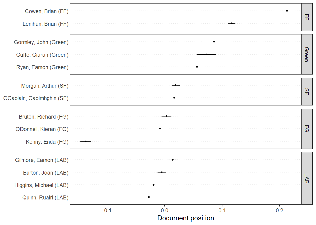
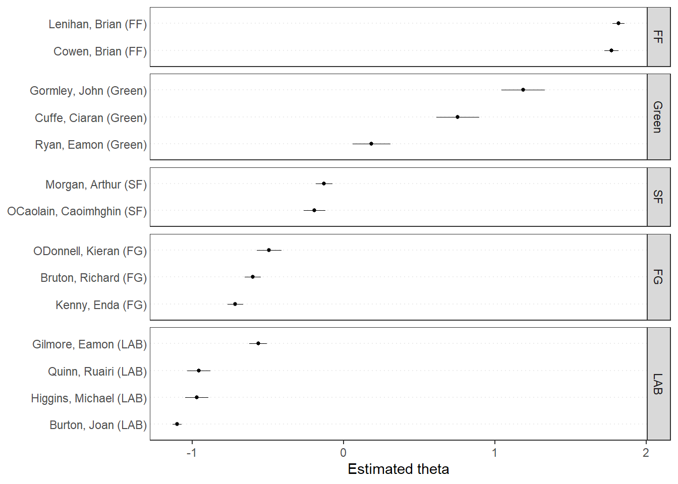
# Get predictionspred <-predict(ws, se.fit =TRUE)# Plot estimated document positions and group by "party" variabletextplot_scale1d(pred, margin ="documents",groups =docvars(data_corpus_irishbudget2010, "party"))
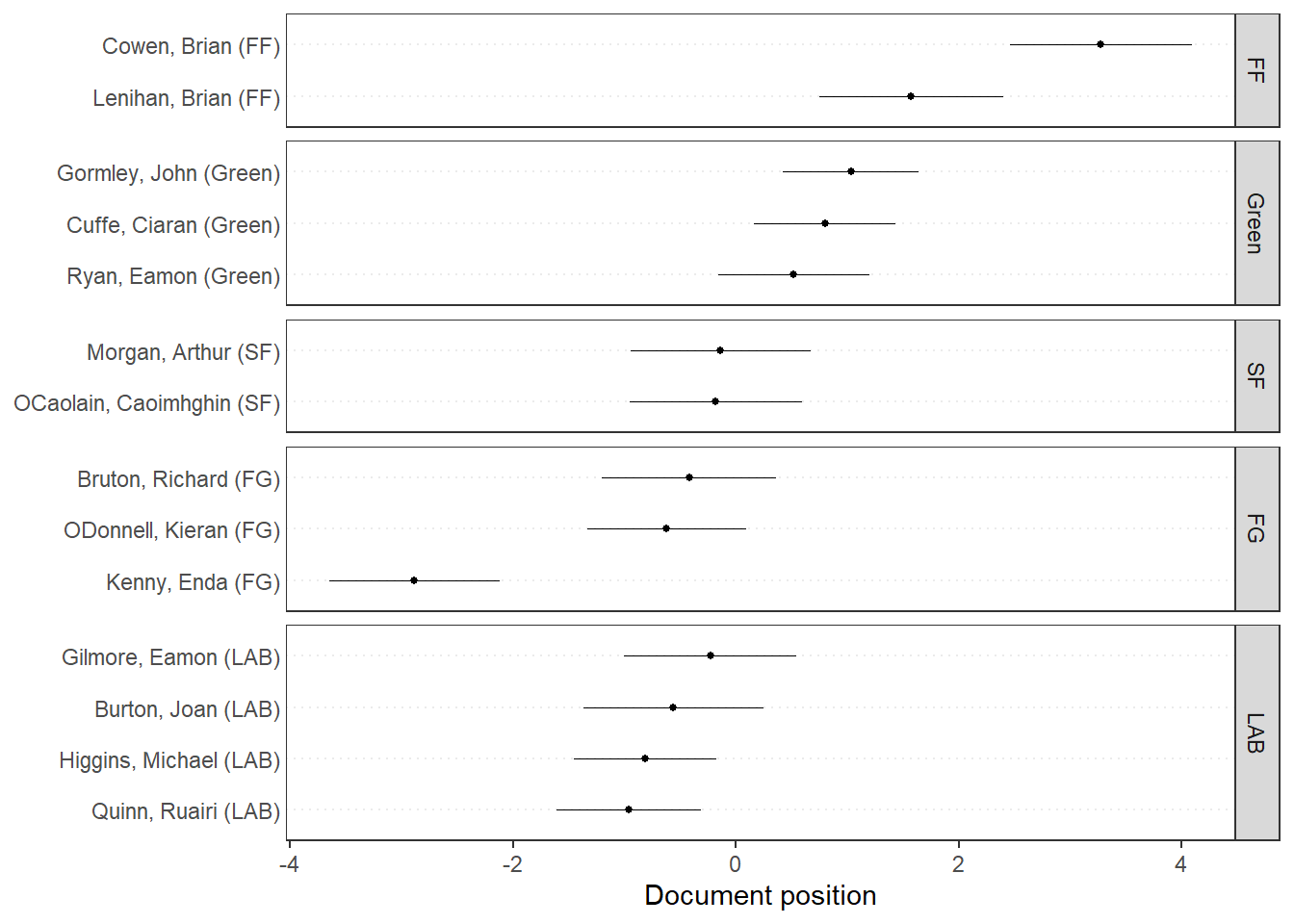
# Plot estimated document positions using the LBG transformation and group by "party" variablepred_lbg <-predict(ws, se.fit =TRUE, rescaling ="lbg")textplot_scale1d(pred_lbg, margin ="documents",groups =docvars(data_corpus_irishbudget2010, "party"))
# Plot estimated document positionstextplot_scale1d(wf, groups = data_corpus_irishbudget2010$party)
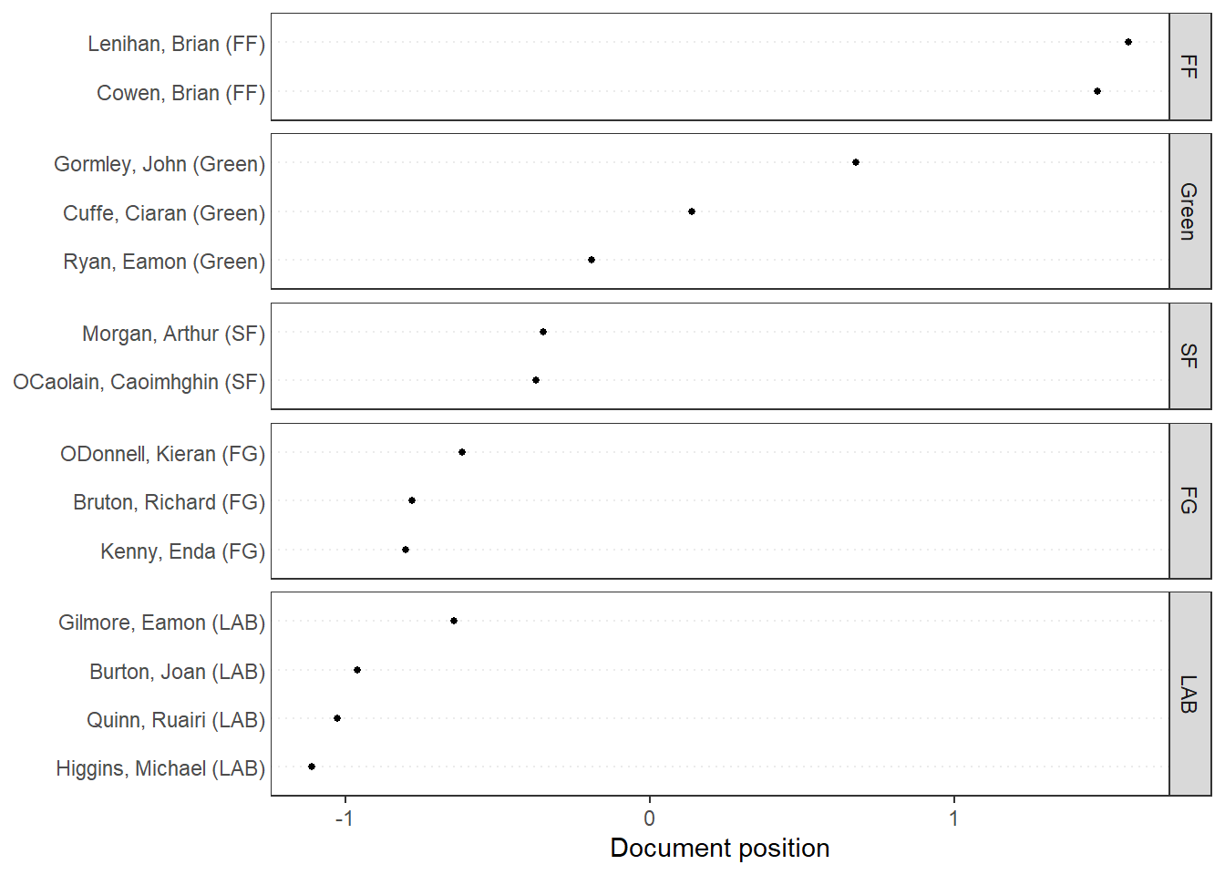
# Transform corpus to dfmie_dfm <-dfm(tokens(data_corpus_irishbudget2010))# Run correspondence analysis on dfmca <-textmodel_ca(ie_dfm)# Plot estimated positions and group by partytextplot_scale1d(ca, margin ="documents",groups =docvars(data_corpus_irishbudget2010, "party"))
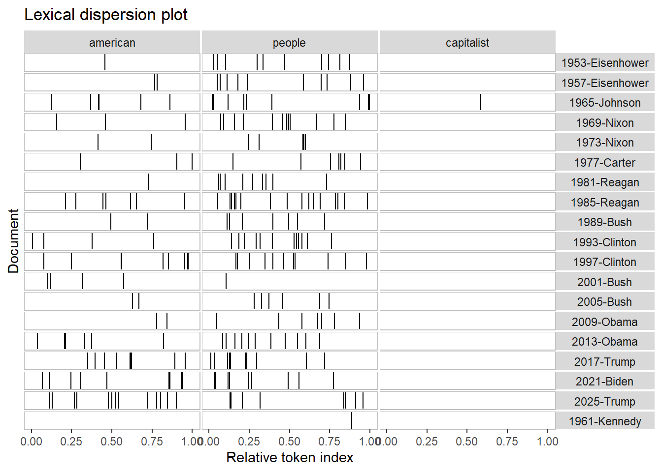
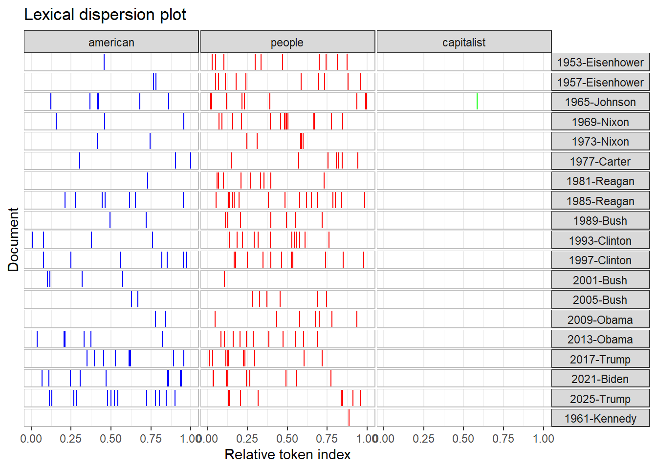
When it comes to the similarities and differences between presidents among time is that some US presidents didn’t use the word “American” too frequent. It became more frequent later because it was used as a key identity during times ,such as World War 2 and the Cold War. After 1949, the terms “American”, and “people” appeared more throughout speeches by US Presidents John F. Kennedy and Ronald Reagan. The term “capitalist”, was less common but more concentrated in specific contexts such as the Cold War.
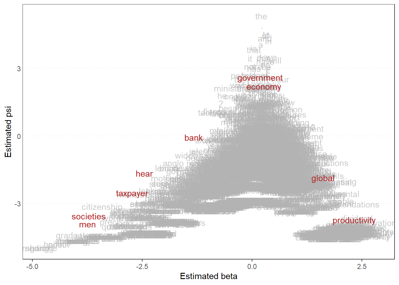
Additionally, the quanteda websites defines Wordfish as a Poisson scaling model that estimates one-dimension document positions that utilizes maximum likelihoods, and both the estimated position of words and the documents can be plotted.