The introduction of Artificial Intelligence started with the release of ChatGBT in November 2022, following other AI model releases such as Google Gemini, Claude, etc. This changed the world especially for data analysts and researchers, being used for research and coding assistance. Questions speculate whether AI can be used to brainstorm and assist with original ideas, or whether it generates the ideas for users.
I argue that AI isn’t a tool to use for generating original ideas; rather that it draws and mixed original and previous research. I also argue that any ideas are completely “original” nowadays, as most of these designs have been publicized before, even though individuals proceed to reinvent and use them in new contexts.
AGI
Google AI defines Artificial General Intelligence (AGI) as a type of technology used for theoretical ways of understanding, learning and performing any intellectual tasks that a human can accomplish. Furthermore, it is programmed to be a research agent, helping to break through scientific research and other disciplines.
I believe that it can be used as a research assistant to produce the best research qualities, but I also argue that it can be used incorrectly, where the model can be prompted to do the research for the user. It may not be completely accurate, but it can be used in an academic dishonest way of conducting research and analyses.
WEEK 2 REFLECTION (2/17/2026): AI AND RESEARCH PROJECT
AI for Knowledge Mining Project
For the group project, me and my colleagues believe we can use AI in our project by helping turn our STATA data zip file to help us use it in RStudio. AI can help us let the data be read in RStudio.
AI Model Selections and Research Applications
We are using ChatGPT and Google Gemini for my project. Some of our colleagues are new using RStudio, so they will ask it to help them if I run into any errors uploading the STATA zip file to RStudio. Additionally, I will help my colleagues with the RStudio and Google Gemini codes to extract our results.
WEEK 3 REFLECTION (2/24/2026): HUMAN KNOWLEDGE, INFORMATION, AND AI DISCREPANCIES/FAILURES
Human Knowledge vs Information
Individuals find and build knowledge based on their experiences and society they grew up in. According to Google AI, key methods of human knowledge are based on logical reasoning, memory, and receiving information from authorities, books, or education.
Knowledge is the capability of a person’s understanding regarding a topic, while information is data a person contains. Information can be transferred, such as an email with a list of documents; it is always kept. Knowledge on the other hand, requires the mental and logical capability to review and understand the data provided. Regarding the email example: a person may keep the email with the listed documents, but the person needs to look at the documents and understand them, which the person may forget.
AI Discrepancies and Failures
AI can create fake and false data/information, such as fake legal cases, political bias, and financial losses due to false predictions. Specifically:
Hallucinations, specifically inventing fake policies or fake news
Embedded Bias and Propaganda: Unfair treatment of women’s rights in Iran and Afghanistan, but portraying as women-friendly nations.
Financial and Strategic Miscalculations: Zillow’s home-buying algorithm overestimated house prices, causing millions of losses and layoffs.
One pattern that makes these discrepancies noticeable is AI-generated information and misinformation; tools used to mislead individuals and causing harm to them.
WEEK 4 REFLECTION (3/3/2026): MACHINE LEARNING PIPELINE ON CYBERCRIME ANALYSIS AND FINANCIAL LOSSES
In this week’s reflection, I created a machine learning pipeline from a cybersecurity incident database that focuses on cyber-attacks on different countries and their financial losses. I specifically focus on:
Number of cyber-crime complaint reports;
Total financial losses from those crimes for 2019 - 2024.
*AI Use Disclaimer: AI tools such as ChatGPT were used as an assistant tool during this reflection to help understand machine learning concepts and code fixture. All analysis, interpretation, and final decisions were reviewed and completed by the author.*
library(tidyverse)
Warning: package 'tidyverse' was built under R version 4.5.3
Warning: package 'ggplot2' was built under R version 4.5.3
Warning: package 'tidyr' was built under R version 4.5.3
Warning: package 'readr' was built under R version 4.5.3
Warning: package 'dplyr' was built under R version 4.5.3
Warning: package 'lubridate' was built under R version 4.5.2
── Attaching core tidyverse packages ──────────────────────── tidyverse 2.0.0 ──
✔ dplyr     1.2.1     ✔ readr     2.2.0
✔ forcats   1.0.0     ✔ stringr   1.5.1
✔ ggplot2   4.0.2     ✔ tibble    3.3.0
✔ lubridate 1.9.4     ✔ tidyr     1.3.2
✔ purrr     1.1.0
── Conflicts ────────────────────────────────────────── tidyverse_conflicts() ──
✖ dplyr::filter() masks stats::filter()
✖ dplyr::lag()    masks stats::lag()
ℹ Use the conflicted package (<http://conflicted.r-lib.org/>) to force all conflicts to become errors
data <-read.csv("C:/Users/akbar/Downloads/LossFromNetCrime.csv",stringsAsFactors =FALSE)# Convert all complaint/loss columns except country to numericnum_cols <-names(data)[names(data) !="Country"]data[num_cols] <-lapply(data[num_cols], function(x) as.numeric(gsub(",", "", x)))str(data)
'data.frame':   117 obs. of  13 variables:
 $ Country         : chr  "PR" "PS" "PT" "PY" ...
 $ X2019_Complaints: num  655 1784 1119 1913 5503 ...
 $ X2019_Losses    : num  5929974 22483591 13870074 10967865 48101706 ...
 $ X2020_Complaints: num  1338 2890 2020 2992 7390 ...
 $ X2020_Losses    : num  7209755 25423219 12391290 13815152 81178182 ...
 $ X2021_Complaints: num  1785 3352 2102 3188 10164 ...
 $ X2021_Losses    : num  9.46e+06 4.89e+07 1.82e+07 2.67e+07 1.32e+08 ...
 $ X2022_Complaints: num  1594 3210 1918 3768 10042 ...
 $ X2022_Losses    : num  1.72e+07 5.78e+07 3.09e+07 4.01e+07 1.87e+08 ...
 $ X2023_Complaints: num  1817 3378 2178 3487 11034 ...
 $ X2023_Losses    : num  2.10e+07 6.93e+07 2.87e+07 3.36e+07 2.44e+08 ...
 $ X2024_Complaints: num  1974 3811 2209 2678 12071 ...
 $ X2024_Losses    : num  3.15e+07 6.60e+07 4.02e+07 4.52e+07 2.81e+08 ...
summary(data)
   Country          X2019_Complaints  X2019_Losses       X2020_Complaints
 Length:117         Min.   :   216   Min.   :2.498e+06   Min.   :   362
 Class :character   1st Qu.:  1119   1st Qu.:1.179e+07   1st Qu.:  1937
 Mode  :character   Median :  5156   Median :4.571e+07   Median :  8187
                    Mean   : 24650   Mean   :2.366e+08   Mean   : 43249
                    3rd Qu.: 16525   3rd Qu.:2.025e+08   3rd Qu.: 28232
                    Max.   :449305   Max.   :3.303e+09   Max.   :796395
  X2020_Losses       X2021_Complaints  X2021_Losses       X2022_Complaints
 Min.   :2.673e+06   Min.   :   391   Min.   :4.363e+06   Min.   :   458
 1st Qu.:1.382e+07   1st Qu.:  2102   1st Qu.:2.286e+07   1st Qu.:  1918
 Median :4.529e+07   Median :  9415   Median :1.000e+08   Median :  8819
 Mean   :2.812e+08   Mean   : 45731   Mean   :4.713e+08   Mean   : 42984
 3rd Qu.:2.125e+08   3rd Qu.: 30367   3rd Qu.:4.003e+08   3rd Qu.: 29642
 Max.   :3.907e+09   Max.   :940125   Max.   :6.467e+09   Max.   :769205
  X2022_Losses       X2023_Complaints  X2023_Losses       X2024_Complaints
 Min.   :6.648e+06   Min.   :   400   Min.   :8.907e+06   Min.   :   330
 1st Qu.:3.350e+07   1st Qu.:  2280   1st Qu.:4.132e+07   1st Qu.:  2253
 Median :1.276e+08   Median :  9527   Median :1.631e+08   Median :  9251
 Mean   :7.196e+08   Mean   : 45505   Mean   :8.590e+08   Mean   : 50734
 3rd Qu.:6.055e+08   3rd Qu.: 31255   3rd Qu.:6.421e+08   3rd Qu.: 31525
 Max.   :1.030e+10   Max.   :876894   Max.   :1.192e+10   Max.   :946966
  X2024_Losses
 Min.   :9.793e+06
 1st Qu.:4.788e+07
 Median :1.876e+08
 Mean   :1.014e+09
 3rd Qu.:8.030e+08
 Max.   :1.446e+10
# Keep only rows with non-missing 2024 lossesdata <- data[!is.na(data$X2024_Losses), ]set.seed(123)n <-nrow(data)train_index <-sample(1:n, size =floor(0.8* n))train <- data[train_index, ]test <- data[-train_index, ]# Variables used in the modelmodel_vars <-c("X2019_Complaints","X2019_Losses","X2020_Complaints","X2020_Losses","X2021_Complaints","X2021_Losses","X2022_Complaints","X2022_Losses","X2023_Complaints","X2023_Losses","X2024_Losses")# Keep only rows without missing valuestrain_model <- train[complete.cases(train[, model_vars]), ]test_model <- test[complete.cases(test[, model_vars]), ]nrow(train_model)
# Compare training vs test errortrain_predictions <-predict(model, newdata = train_model)train_rmse <-sqrt(mean((train_predictions - train_model$X2024_Losses)^2))test_rmse <-sqrt(mean((predictions - test_model$X2024_Losses)^2))train_rmse
[1] 98847983
test_rmse
[1] 406916980
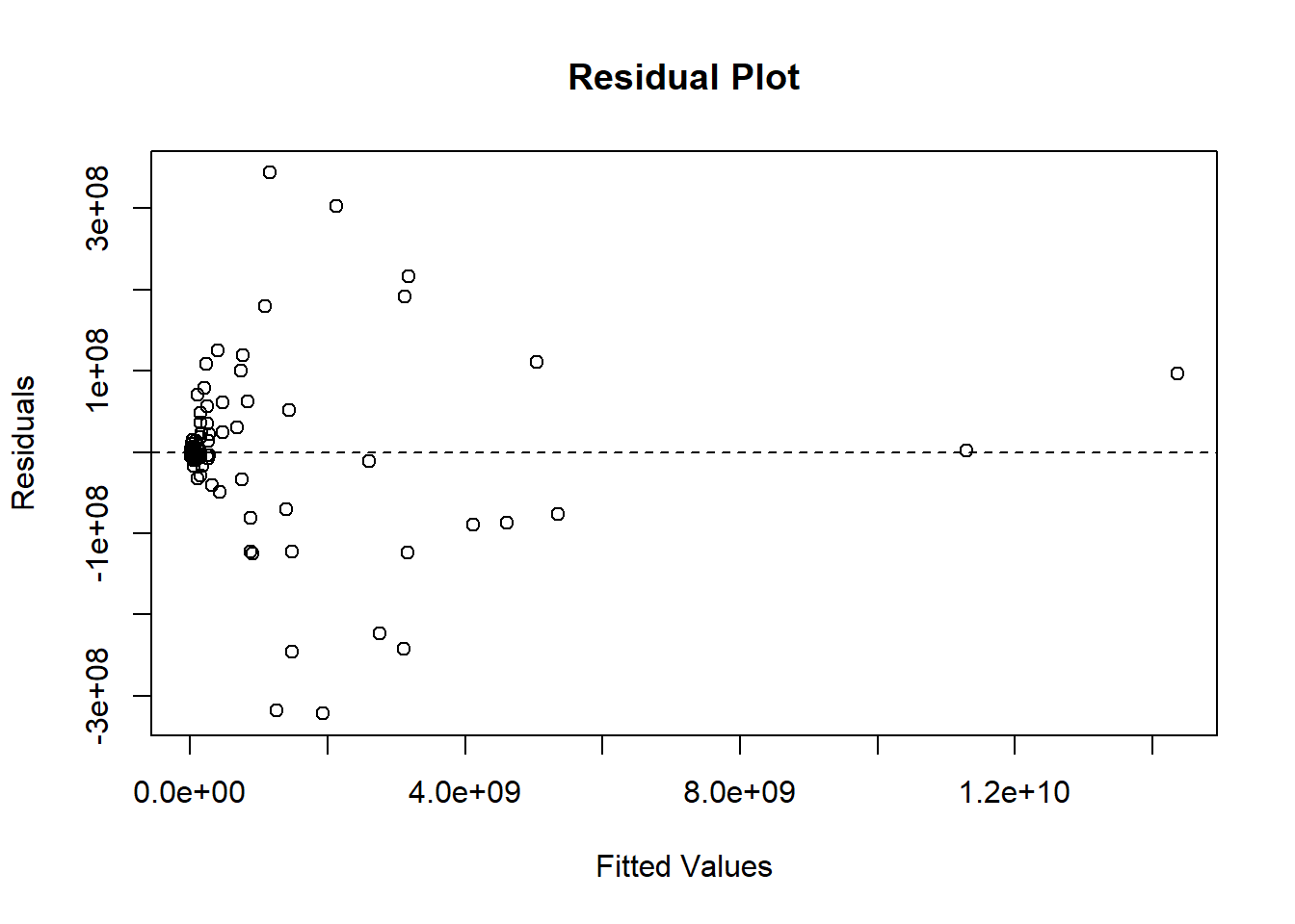
# Looking at residuals to help with error analysisplot(model$fitted.values, model$residuals,xlab ="Fitted Values",ylab ="Residuals",main ="Residual Plot")abline(h =0, lty =2)
# Checking actual vs predicted plotsresults <-data.frame(Actual = test_model$X2024_Losses,Predicted = predictions)head(results)
The dataset is first imported and cleaned by removing rows with missing outcome values and converting the complaint and loss variables to numeric format. Following after, since the dataset contains too much data I split it into training and testing sets, which led to a linear regression being trained on the training data. The predictions are generated for the test data, and model performance is reviewed using Root Mean Squared Error (RMSE).
For the error analysis, the RMSE reveals how the model behaved across observations through the comparison of training vs testing errors. The residual plot demonstrates whether the model prediction errors followed any over or under-predicted losses.
Overfitting focuses on the differences between learning knowledge and learning noise in the data. When it comes to overfitting, a model can capture random fluctuations in the training data instead of generalizing patterns.
WEEK 5 REFLECTION (3/10/2026): PREDICTION VS EXPLANATION, SIMPLE CAUSAL RELATIONSHIP DIAGRAM AND DIFFERENTIATING CAUSAL VS PREDICTIVE CLAIMS:
Prediction matters when there’s is a clear goal or forecasting something accurately. When a policymaker wants to predict how to reduce crime and poverty in a state, they outline their ideas and pass a policy or law in hopes of producing an effective outcome.
Explanation matters when something happens and therefore needs to be a reason or a statement supporting the outcome. When a law or policy has been passed, the policymaker gives his/her reasoning why it’s effective. Prediction is the foreshadowing of an event, whereas an explanation is the reasoning or conclusion of the prediction taking place.
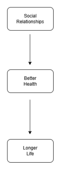
For the diagram above, the co-founders are variables that could affect both social relationships and health. Such variables could be age, income/socioeconomic status, education, access to healthcare, lifestyle and mental health.
For distinguishing a causal claim from a predictive association, a causal claim would be just like the causal diagram above. A predictive association would only indicate that individuals with stronger relationship skills tend to have better health and longer lives, without social relationships being the reason.
WEEK 6 REFLECTION (3/17/2026): TEXT MINING, NLP, LLM, AND AI FOR RESEARCH GUIDE
Google AI Overview states that text-mining, often referred to as “distant reading,” excels at identifying broad patterns, trends, and structures across extensive datasets – such as numerous books or millions of social media posts – that are impossible for a person to read. While close reading focuses on interpreting individual texts to find detailed qualitative meaning, text-mining provides a data-focused perspective of textual patterns. The blind spots however, include context, irony, and the nuanced interpretation of low-probability words.
Natural Language Processing (NLP) and Large Language Models (LLM) can assist in research by analyzing a vast number of unstructured datasets and accelerate them through routine tasks. An example of this scenario is a data analyst having unorganized datasets (papers, documents, files), and using these models to organize, clean up its unnecessary parts and complete them at a faster rate.
Google AI Overview states NLP and LLM models having a couple of limitations, such as generating false information, having the inability to reason logically, and having a lack of real-time knowledge. Suggested solutions include clear prompt-engineering, specifically providing the models clear instructions through specific prompts. Another suggestion is through Retrieval-Augmented Generation (RAG), which helps providing external knowledge and hybrid approaches, combining traditional NLP with LLM together.
AI For Research Guide
Note: My ideas for this AI Research Guide were informed in part by Harvard’s Library Artificial Intelligence for Research and Scholarship guide.
AI can help researchers discover literature, summarize key points and trends.
It can break down large pieces of information into smaller portions.
AI can assist with analyzing, clarifying and editing data and content.
AI-generated information should be always verified by multiple reliable sources.
It is encouraged to use AI for literature research when looking for new resources.
Citation References:
“Research Guides: Artificial Intelligence for Research and Scholarship: AI for Research.” 2026. AI for Research - Artificial Intelligence for Research and Scholarship - Research Guides at Harvard Library. Accessed March 4, 2026. https://guides.library.harvard.edu/c.php?g=1330621&p=10034534
WEEK 7 REFLECTION (3/24/2026): LLM FAILURES, AI IN THE FUTURE
According to Google AI Overview, LLMs exceed in text mining, summarizing information, and coding. However, they lack in high accuracy tasks, logical reasoning, updated knowledge, and have a limited understanding of the real world. When I first gave ChatGPT a prompt for a project I was working on, it understood the general requirements, but the code it generated was incorrect in the first couple of attempts. After I provided my working directory and database structure, the model was able to produce the correct code and assist me more effectively.
With my pursuit of becoming a data analyst/scientist in the next five years, generative AI can help me in the future with coding assistance, breaking down big portions of information into smaller bits, and editing data. I believe that AI isn’t and shouldn’t take over the data industry, since data-review and verification needs to be hand-operated. AI can and will be helpful for coding assistance and visualization, but the originality, creativity and ideas need to remain human-driven.
WEEK 8 REFLECTION (3/31/2026): RAG CRITICISMS AND IMPROVEMENTS
According to Google AI Overview, RAG (Retrieval-Augmented Generation) is an AI framework that LLM outputs by referencing internal documents or the internet before generating a response, which matters for research since it stays up-to-date, reduces hallucinations, specializes data, information, and offers cited and verified facts.
Grounding generation in retrieved documents change the trustworthiness of AI output through verifying evidences, reducing misinformation, being contextually accurate, and having AI easily explaining it with increased confidence in the output.
Some criticisms of RAG include inaccuracies and unreliability, as well as delivering outdated or incomplete information.
In order to improve generation is through advanced retrieval techniques, data preparation & chunking.
WEEK 9 REFLECTION (4/7/2026): KNOWLEDGE GRAPHS, WITH ITS NODES AND RELATIONSHIPS
Google Gemini states that a knowledge graph is a structured representation of information that models as a network of connected entities and relationships.
It differs from a traditional database and vector store because its data structure is made of of nodes (entities) and edges (relations), whereas traditional (relational) databases contains rows and columns, and vector store contain high-dimensional numerical arrays.
The reason why relationships between entities for knowledge mining are valuable is due to multiple factors: contextual disambiguation, inference and reasoning, pattern and path discovery, and enhancing AI accuracy, which is done through RAG.
In terms of a social data analyst perspective, three nodes could be neighborhoods, ZIP codes and specific metropolitan areas, and three relationships could be neighborhoods being located within ZIP codes, which is part of a metropolitan zone. The reason why this structure helps answer question a flat dataset cannot is due to flat datasets being built for direct attributes, whereas knowledge graphs are built for indirect paths.
WEEK 10 REFLECTION (4/14/2026): AI FOR SCIENCE AND AGENTIC AI SYSTEMS
ChatGPT defines AI for Science as the utilization of Artificial Intelligence to help with making scientific discoveries, where it helps scientists with data analysis, organization, cleaning, and solving complex model systems.
Agentic AI systems are designed to be efficient research assistants compared to single-prompt interactions., where it can manage breaking tasks into smaller parts, analyze outcomes, revise strategies and proceeds to work through the problems with stages.